Baseline model

We begin with a linearized, three-equation New Keynesian model with one productivity shock. This is the first example in the paper. We learn its policy functions and likelihood with neural networks, then extend it step by step.

NoteA faster version for class

rank_baseline_fast.py trains the same model in about seven minutes on a laptop CPU, with a smaller batch and fewer likelihood draws. Its solution is less precise.

View notebook on GitHub

Model

The model is log-linearized around its steady-state equilibrium,

\[ \begin{aligned} \hat X_t &= E_t\hat X_{t+1} -\sigma^{-1}\left(\phi_\Pi\hat\Pi_t+\phi_Y\hat X_t-E_t\hat\Pi_{t+1}-\hat R_t^*\right),\\ \hat\Pi_t &= \kappa\hat X_t+\beta E_t\hat\Pi_{t+1},\\ \hat R_t^* &= \rho_A\hat R_{t-1}^* +\sigma(\rho_A-1)\omega\sigma_A\epsilon_t^A. \end{aligned} \]

Here \(\hat X_t\) is the output gap, \(\hat\Pi_t\) is inflation’s deviation from steady state, and \(\hat R_t^*\) is the natural-rate deviation. The natural rate follows the exogenous process implied by the productivity shock. The coefficients are

\[\kappa=\frac{(1-\phi)(1-\phi\beta)(\sigma+\eta)}{\phi},\qquad \omega=\frac{1+\eta}{\sigma+\eta}.\]

Neural network solution

Formulation

Following the general form in Section 2.2 of the paper, the state, shock, and policy functions are

\[ \mathbb S_t=\{\hat R_t^*\},\qquad \nu_t=\{\epsilon_t^A\},\qquad \psi_t=\{\hat X_t,\hat\Pi_t\}. \]

All eight parameters vary during training and are available for estimation, so the calibrated set is empty,

\[ \tilde\Theta=\{\beta,\sigma,\eta,\phi,\phi_\Pi,\phi_Y,\rho_A,\sigma_A\}, \qquad \bar\Theta=\varnothing. \]

The neural network learns output and inflation as functions of the state and parameters,

\[ \begin{pmatrix}\hat X_t\\\hat\Pi_t\end{pmatrix} =\psi_{NN}(\mathbb S_t,\tilde\Theta\mid\bar\Theta). \]

We train it on the errors in the two equilibrium equations,

\[ \begin{aligned} F_1 &= \hat X_t-\left[E_t\hat X_{t+1} -\sigma^{-1}\left(\phi_\Pi\hat\Pi_t+\phi_Y\hat X_t-E_t\hat\Pi_{t+1}-\hat R_t^*\right)\right],\\ F_2 &= \hat\Pi_t-\left(\kappa\hat X_t+\beta E_t\hat\Pi_{t+1}\right). \end{aligned} \]

The loss is the weighted mean of the squared equation errors over a training batch,

\[ \mathcal L=\frac{1}{N_{batch}}\sum_{b=1}^{N_{batch}}\sum_{j}\alpha_j\left(F_j^{(b)}\right)^2. \]

Here \(N_{batch}\) is the number of simulated economies in a training batch and \(F_j^{(b)}\) is equation \(j\)’s residual for economy \(b\). As in the replication, both equation weights are \(\alpha_1=\alpha_2=1000\). Training settings explains why.

In the code

Parameters, ranges, and shocks

PARAMETERS holds the reference calibration, which also generates the data later on. RANGES gives the distribution from which each parameter is drawn during training. Because every parameter has a range, all eight are pseudo-state variables that enter the network as inputs. SHOCKS gives the distribution of the productivity innovation.

examples/rank/rank_baseline.py

# Reference values. They also generate the data later on.
PARAMETERS = {
    "beta": 0.97,
    "sigma": 2.0,
    "eta": 1.125,
    "phi": 0.7,
    "phipi": 1.875,
    "phiy": 0.25,
    "rho_a": 0.875,
    "sigma_a": 0.06,
}

# Training ranges. Every parameter with a range is a network input.
RANGES = {
    "beta": torch.distributions.Uniform(0.95, 0.99),
    "sigma": torch.distributions.Uniform(1.0, 3.0),
    "eta": torch.distributions.Uniform(0.25, 2.0),
    "phi": torch.distributions.Uniform(0.5, 0.9),
    "phipi": torch.distributions.Uniform(1.25, 2.5),
    "phiy": torch.distributions.Uniform(0.0, 0.5),
    "rho_a": torch.distributions.Uniform(0.8, 0.95),
    "sigma_a": torch.distributions.Uniform(0.02, 0.1),
}

# Distributions of the shock innovations.
SHOCKS = {"zeta": torch.distributions.Normal(0.0, 1.0)}

The model class

NKModel collects the model. POLICY_NAMES and STATE_NAMES fix the order of the network’s outputs and state inputs. The natural rate \(\hat R_t^*\) is called zeta, and the learned policies are X and Pi. RESIDUAL_NAMES and RESIDUAL_LABELS name the equation errors in the order \(F_1\), \(F_2\). The constructor stores the parameters, their ranges, and the shocks, and builds the network. The remaining attributes hold the simulated economies during training and the training history.

examples/rank/rank_baseline.py

class NKModel:
    """The network learns X and Pi. The Taylor rule is substituted into the Euler equation."""

POLICY_NAMES = ("X", "Pi")
STATE_NAMES = ("zeta",)
# Equation residuals, in the order of the equations above.
RESIDUAL_NAMES = ("res_bond_euler", "res_nkpc")
RESIDUAL_LABELS = ("Euler equation", "Phillips curve")

def __init__(self, parameters, ranges, shocks, seed=1234):
    seed_all(seed)
    self.par = Parameters(parameters)
    self.ranges = Ranges(parameters, ranges)
    self.shocks = Shocks(shocks)
    self.network = self.make_network()
    self.par_draw = self.ss = self.state = None
    self.loss_dict = self.training_conf = None

From states to policies

make_network builds the network. Its first layer maps every input to \([-1, 1]\), using state_bounds for the natural rate and the training range for each parameter. Five hidden layers of 64 CELU units follow, then a linear layer with one output per policy.

examples/rank/rank_baseline.py

def state_bounds(self):
    return torch.tensor([-0.025]), torch.tensor([0.025])

def make_network(self, hidden=64, layers=5, activation=torch.nn.CELU):
    """Normalize states and parameters, then apply a fully connected network."""
    layer_list = []

    # Normalize layer
    state_low, state_high = self.state_bounds()
    low = torch.cat((state_low, self.ranges.low_tensor()))
    high = torch.cat((state_high, self.ranges.high_tensor()))
    layer_list.append(NormalizeLayer(low, high))

    # First layer
    layer_list.append(torch.nn.Linear(len(low), hidden))
    layer_list.append(activation())

    # Middle layers
    for _ in range(1, layers):
        layer_list.append(torch.nn.Linear(hidden, hidden))
        layer_list.append(activation())

    # Last layer
    layer_list.append(torch.nn.Linear(hidden, len(self.POLICY_NAMES)))

    return torch.nn.Sequential(*layer_list)

policy combines the states and parameters and passes them to the network. The same method also evaluates policies at future states, which we need for expectations. After evaluating the network, we assign its output columns to X and Pi and divide each prediction by 100, which scales the network outputs to small model deviations.

examples/rank/rank_baseline.py

def policy(self, state=None, par=None):
    state = self.state if state is None else state
    par = self.par_draw if par is None else par

    # Vectors of states and parameters.
    states = state.cat(keys=self.STATE_NAMES)
    parameters = par.cat()

    # Future states have an extra leading dimension for the shock draws.
    # Repeat the parameters along it to evaluate expectations.
    if states.dim() > parameters.dim():
        parameters = parameters.expand(states.shape[0], *parameters.shape)

    # Evaluate the network on the combined inputs.
    inputs = torch.cat((states, parameters), dim=-1)
    output = self.network(inputs)

    X = output[..., 0:1] / 100
    Pi = output[..., 1:2] / 100

    return X, Pi

Construct next-period states

To evaluate future policies, we first need future states. next_state uses the current state in self.state, the parameters in self.par_draw, and the shock draws in e. Here e.zeta contains the standard-normal productivity innovations \(\epsilon_{t+1}^A\), and self.ss.omega is \(\omega=(1+\eta)/(\sigma+\eta)\).

The method writes out the natural-rate transition from the model equations and returns the next-period values in a State container. It leaves today’s state unchanged so we can compare current policies with expected future policies.

examples/rank/rank_baseline.py

@torch.no_grad()
def next_state(self, e):
    """Return next period's state for the shock draws in e, without changing the current state."""
    par = self.par_draw
    loading = par.sigma_a * par.sigma * (par.rho_a - 1) * self.ss.omega
    zeta_next = par.rho_a * self.state.zeta + loading * e.zeta
    return State({"zeta": zeta_next})

From policies to equation errors

We train without target values for output and inflation. Instead, the model’s equations check the network’s predictions. We first evaluate today’s policies, then the policies at simulated future states. Averaging over the shock draws approximates the conditional expectations in the equations.

examples/rank/rank_baseline.py

def residuals(self, e, detach_next=True):
    par = self.par_draw

    # Evaluate today's policies.
    X, Pi = self.policy()

    # Next period's state for each shock draw.
    state_next = self.next_state(e)

    # Evaluate next period's policies at that state.
    with torch.set_grad_enabled(not detach_next):
        X_next, Pi_next = self.policy(state_next)

    # Average over the draws to approximate the conditional expectations.
    EX_next = X_next.mean(dim=0)
    EPi_next = Pi_next.mean(dim=0)

    # Substitute the Taylor rule into the Euler equation.
    I = par.phipi * Pi + par.phiy * X

    # F_1: Euler equation.
    euler = X - (EX_next - (I - EPi_next - self.state.zeta) / par.sigma)
    # F_2: Phillips curve.
    phillips = Pi - (self.ss.kappa * X + par.beta * EPi_next)
    return [euler, phillips]

The same network produces today’s and next period’s policies. With detach_next=True, as in these examples, next period’s predictions are held fixed and only today’s predictions move toward them. With detach_next=False, as in the paper, the gradient also accounts for how an update moves next period’s policies. Holding them fixed is cheaper and more stable, but ignores part of the gradient. In both cases the training loop below repeats the update inner_steps times on the same states. Each repetition draws new shocks and recomputes the expectations with the updated network, so today’s policies and their expected future values can settle together before the economy moves on.

From equation errors to a loss

At equilibrium, each residual is zero. The loss squares the residuals, averages them over the training batch, and adds the two equation losses with weights \(\alpha_j\). This is a weighted mean squared error. The weights follow the residual order, \(F_1\) for the Euler equation and then \(F_2\) for the Phillips curve. The method also returns the unweighted equation losses for the training history and plots.

examples/rank/rank_baseline.py

def loss(self, residuals, weights):
    """Return the weighted mean squared error and each unweighted equation loss."""
    equation_losses = [residual.square().mean() for residual in residuals]
    loss = sum(weight * value for weight, value in zip(weights, equation_losses))
    components = {name: value.item() for name, value in zip(self.RESIDUAL_NAMES, equation_losses)}
    return loss, components

The training loop

train_model puts the pieces together. It draws a batch of parameter vectors, and prepare starts each economy from the stationary distribution of the natural rate. Each iteration then follows six steps.

1. Run the inner loop. It takes inner_steps gradient updates while the states and parameters stay fixed. Each update draws mc new shocks as antithetic pairs, computes the residuals and the loss, backpropagates, clips the gradient norm at one, and lets AdamW change the network weights.
2. Record the equation losses of the first update.
3. Update the equation weights. Fixed weights stay unchanged.
4. Update the learning rate along the cosine schedule.
5. Redraw the parameters every par_draw_after iterations.
6. Simulate every economy forward by config.steps periods with steps. This gives the states for the next iteration.

Redrawing parameters and simulating forward means the network sees states and parameter values where the economy actually spends its time.

examples/rank/rank_baseline.py

def prepare(self, par_draw, batch, device="cpu"):
    self.par_draw = par_draw.to(device)
    self.ss = self.steady_state()
    self.state = self.initialize_state(batch=batch, device=device)

examples/rank/rank_baseline.py

def train_model(self, config):
    """Train the policy network with the settings in config."""
    seed_all(config.seed)
    self.training_conf = config

    # Set the network to train mode.
    self.network.train()
    self.to(config.device)

    # Draw parameters and initial states.
    par_draw = self.draw_parameters((config.batch, 1), device=config.device)
    self.prepare(par_draw, batch=config.batch, device=config.device)

    # Starting weights for the equations.
    weights = config.weights.initial(len(self.RESIDUAL_NAMES))
    weight_state = None

    # Optimizer and scheduler.
    optimizer = torch.optim.AdamW(self.network.parameters(), lr=config.lr)
    scheduler = torch.optim.lr_scheduler.CosineAnnealingLR(
        optimizer, T_max=config.iteration, eta_min=config.min_lr)

    # Loss history: the total, each equation, and each equation weight.
    self.loss_dict = {"iteration": [], "total": []}
    for name in self.RESIDUAL_NAMES:
        self.loss_dict[name] = []
        self.loss_dict[f"w_{name}"] = []

    # Training loop.
    pbar = trange(config.iteration)
    running_loss = 0.0
    for i in pbar:
        # Update the network several times on the same states, with new shocks each time.
        for o in range(config.inner_steps):
            optimizer.zero_grad()
            shape = (config.mc, config.batch, 1)
            e = self.draw_shocks(shape, antithetic=True, device=config.device)
            residuals = self.residuals(e, config.detach_next)
            loss, components = self.loss(residuals, weights)
            loss.backward()
            torch.nn.utils.clip_grad_norm_(self.network.parameters(), 1.0)
            optimizer.step()

            # Record the first update, before the network adapts to these states.
            if o == 0:
                self.loss_dict["iteration"].append(i)
                self.loss_dict["total"].append(loss.item())
                for name, weight in zip(self.RESIDUAL_NAMES, weights):
                    self.loss_dict[name].append(components[name])
                    self.loss_dict[f"w_{name}"].append(weight)
                running_loss += loss.item()

        # Update adaptive weights. Fixed weights stay unchanged.
        losses = list(components.values())
        weights, weight_state = config.weights.update(
            weights, losses, i, warmup_iter=None, state=weight_state)

        # Show the running loss in the progress bar.
        if i % config.print_after == 0:
            pbar.set_postfix({
                "loss": running_loss / config.print_after,
                "lr": scheduler.get_last_lr()[0],
            })
            running_loss = 0.0

        # Update the learning rate.
        scheduler.step()

        # Draw new parameters.
        if i % config.par_draw_after == 0:
            self.par_draw = self.draw_parameters((config.batch, 1), device=config.device)
            self.ss = self.steady_state()

        # Sample new states by simulation.
        self.steps(config.batch, config.device, config.steps)

    # Set the network to evaluation mode.
    self.network.eval()
    self.to("cpu")

Simulate the economies

step moves the economies one period with the shock draws in e and returns the realized variables. The order of the two moves matters. During training, steps calls it with advance_first=False, so the policies are evaluated at the current state, as in residuals, before the state moves. The particle filter calls forecast, which uses advance_first=True. The state moves first and the policies are evaluated at the new state, which is the order a bootstrap particle filter needs. Both steps and forecast also accept fixed shock sequences instead of fresh draws, which makes simulations and likelihood evaluations repeatable.

examples/rank/rank_baseline.py

@torch.no_grad()
def step(self, e, advance_first=True):
    """Move the economies one period and return the realized variables.

    With advance_first=True (particle filter and simulation), the state moves first and the
    policies are evaluated at the new state. With advance_first=False (training), they are
    evaluated at the current state, consistent with residuals.
    """
    state_next = self.next_state(e)
    state = state_next if advance_first else self.state
    X, Pi = self.policy(state)
    self.state = state_next
    return {"R": state.zeta, "X": X, "Pi": Pi}

def steps(self, batch, device, steps, shocks=None):
    """Simulate the training economies. shocks (name -> (steps, batch, 1)) replaces fresh draws."""
    for t in range(steps):
        if shocks is None:
            e = self.draw_shocks((batch, 1), device=device)
        else:
            e = Element({key: value[t] for key, value in shocks.items()})
        self.step(e, advance_first=False)

Training settings

TrainingConfig collects the settings for the training loop. The script trains the network with the following call, or loads the saved one.

examples/rank/rank_baseline.py

model = NKModel(PARAMETERS, RANGES, SHOCKS)
model_path = folder / "model.pt"
train_model = not load_model or not model_path.exists()

training_config = TrainingConfig(
    iteration=10000,
    inner_steps=5,
    steps=10,
    batch=500,
    mc=2,
    par_draw_after=1,
    lr=1e-3,
    min_lr=1e-10,
    device=DEVICE,
    seed=1234,
    weights=ConstantWeights([1000.0, 1000.0]),
    detach_next=True,
)

if train_model:
    print("Training the policy network...")
    model.train_model(training_config)
    # A new policy needs new observations, so delete the saved ones.
    (folder / "observations.pt").unlink(missing_ok=True)
    model.save(model_path)
else:
    print("Loading the saved policy network.")
    model.load(model_path)

Each update uses a batch of 500 economies and mc=2 draws, a single antithetic pair of shocks. The model is linear, so the pair already gives close approximations of the expectations. Extension 8 raises the number of draws.

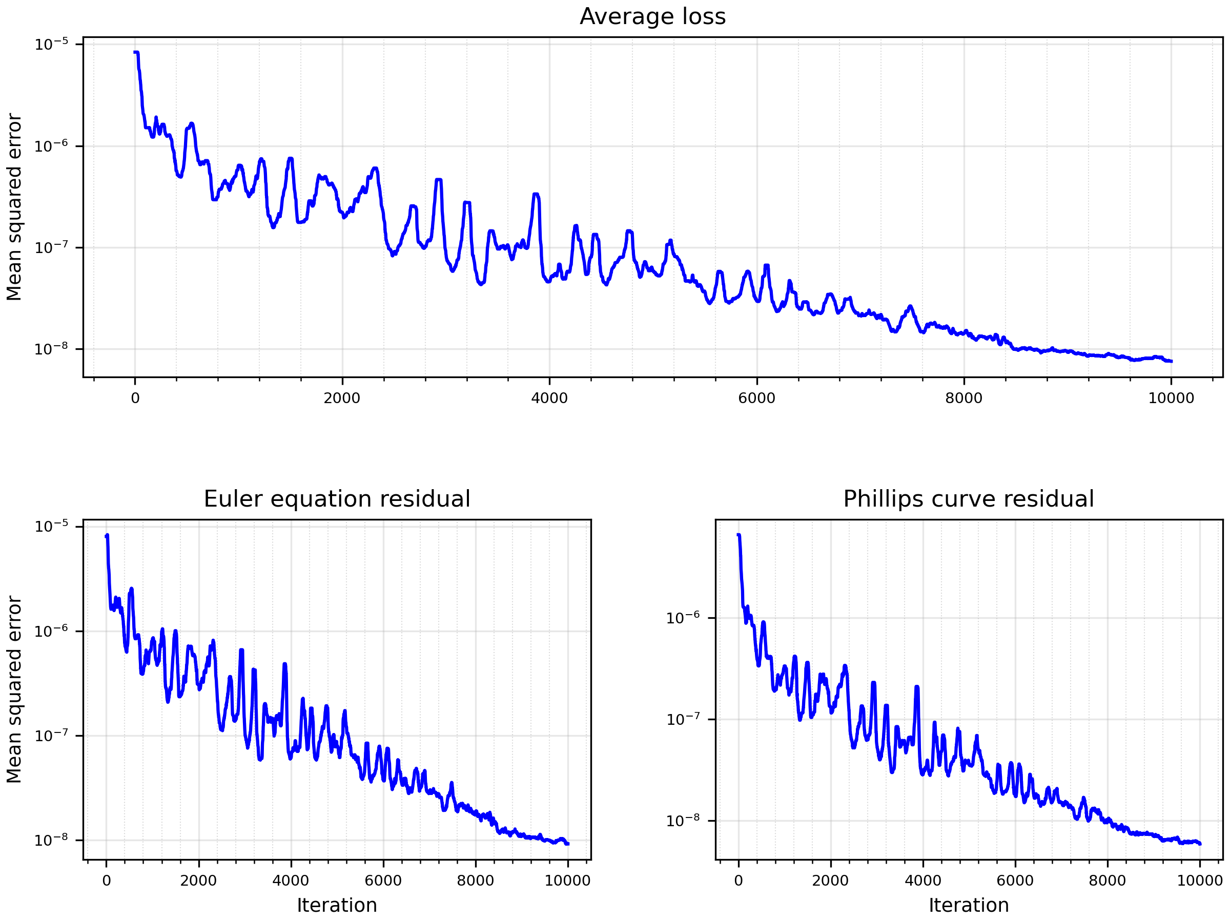
ConstantWeights fixes both equation weights at 1,000. The scale matters for the optimizer, not for the solution. Once the network is accurate, the mean squared residuals are around \(10^{-8}\). Most of their gradients then fall below the \(\epsilon=10^{-8}\) that AdamW adds to its step-size denominator, so the updates shrink and training stalls. Multiplying the loss by 1,000 keeps the gradients well above \(\epsilon\). The replication package uses the same factor.

ReLoBRaLo instead adapts the weights during training. Both the equation losses and the weights are recorded. Set load_model = False to train with changed settings.

Results

Mean squared residuals during training, with their average on top and each equation below, smoothed by a moving median over 100 iterations.

Output gap \(\hat X_t\) as each estimated parameter varies, the others at reference values, after a productivity innovation of minus one standard deviation. The dashed line is the analytical solution.

Inflation \(\hat\Pi_t\) as each estimated parameter varies.

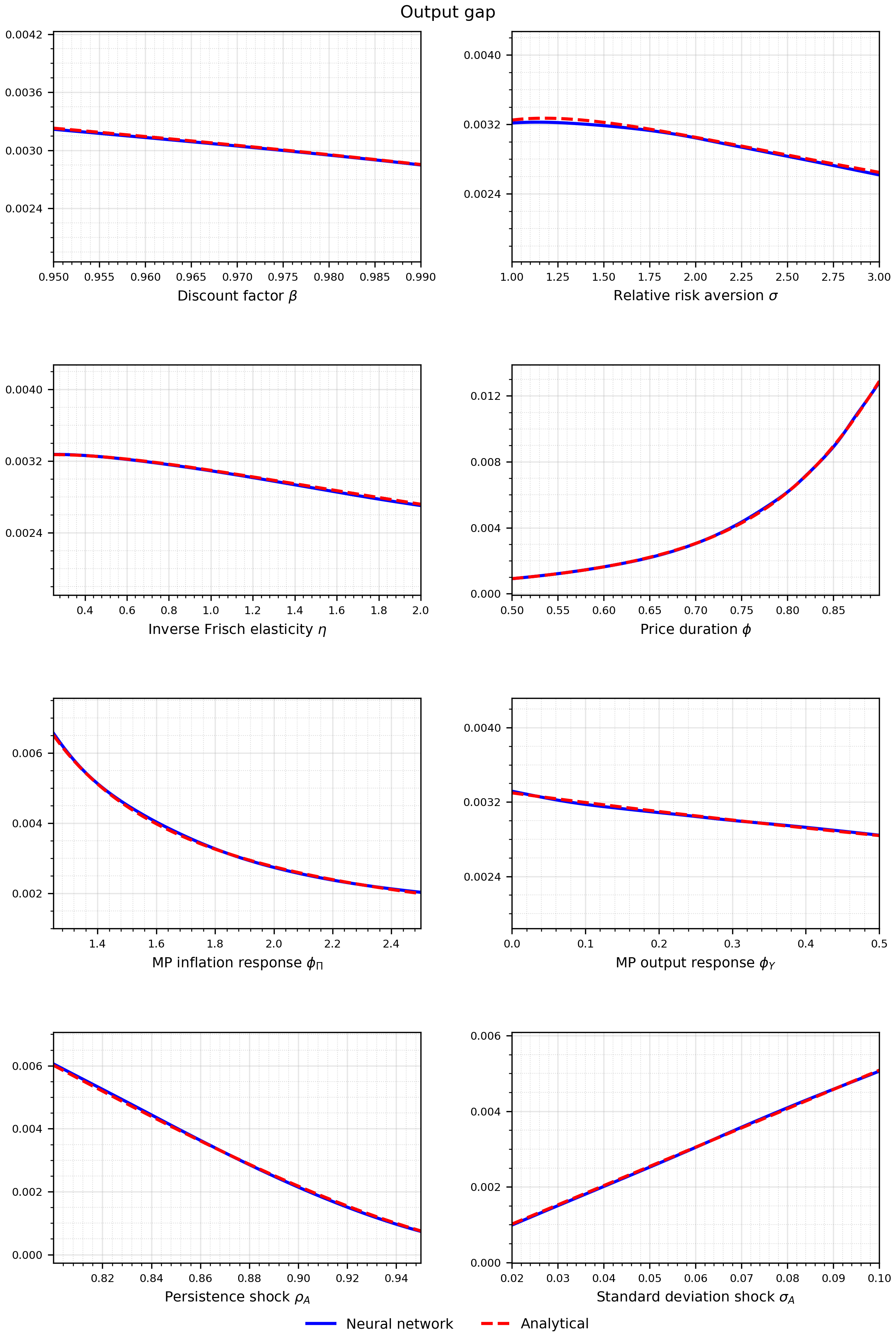
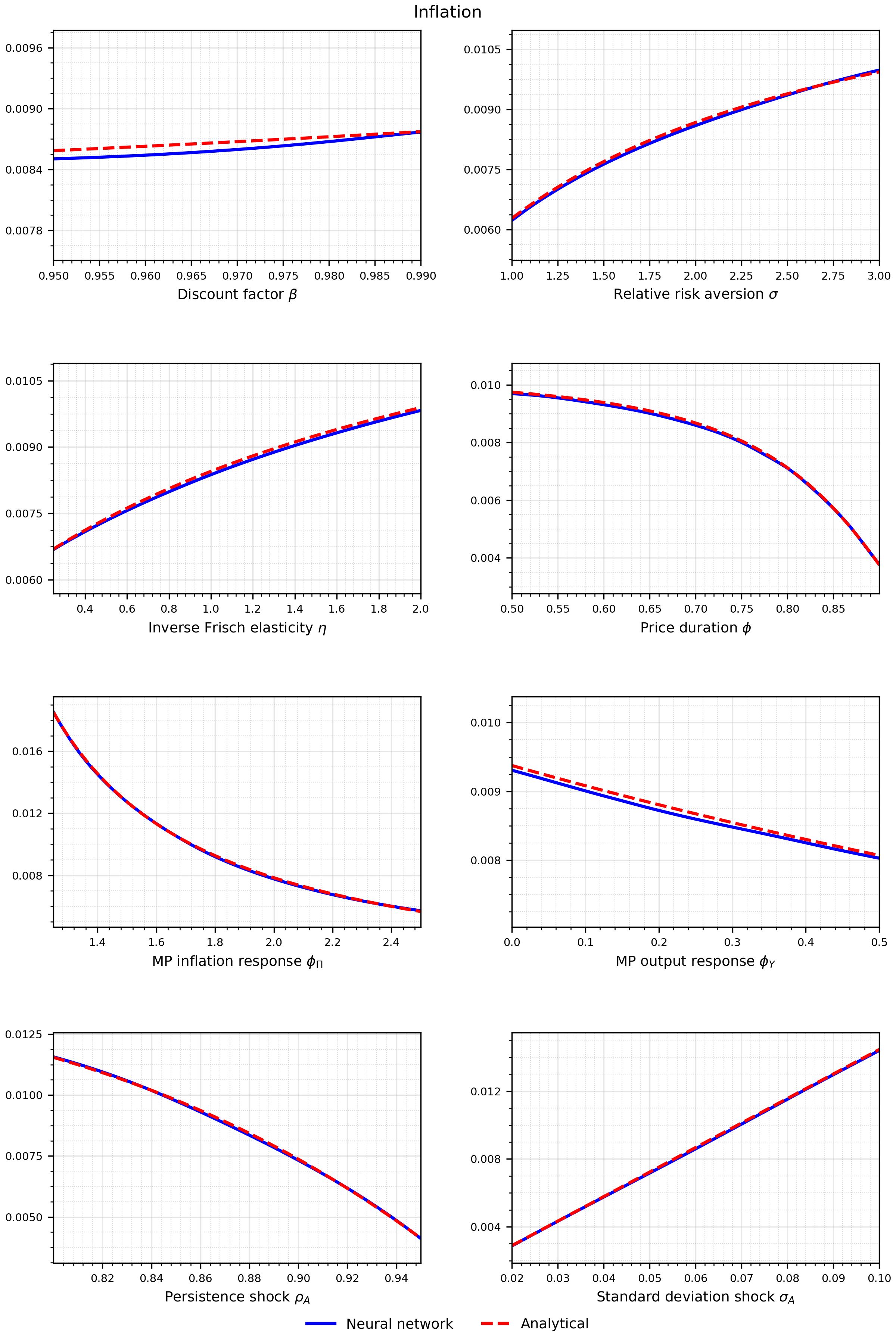
Likelihood approximation

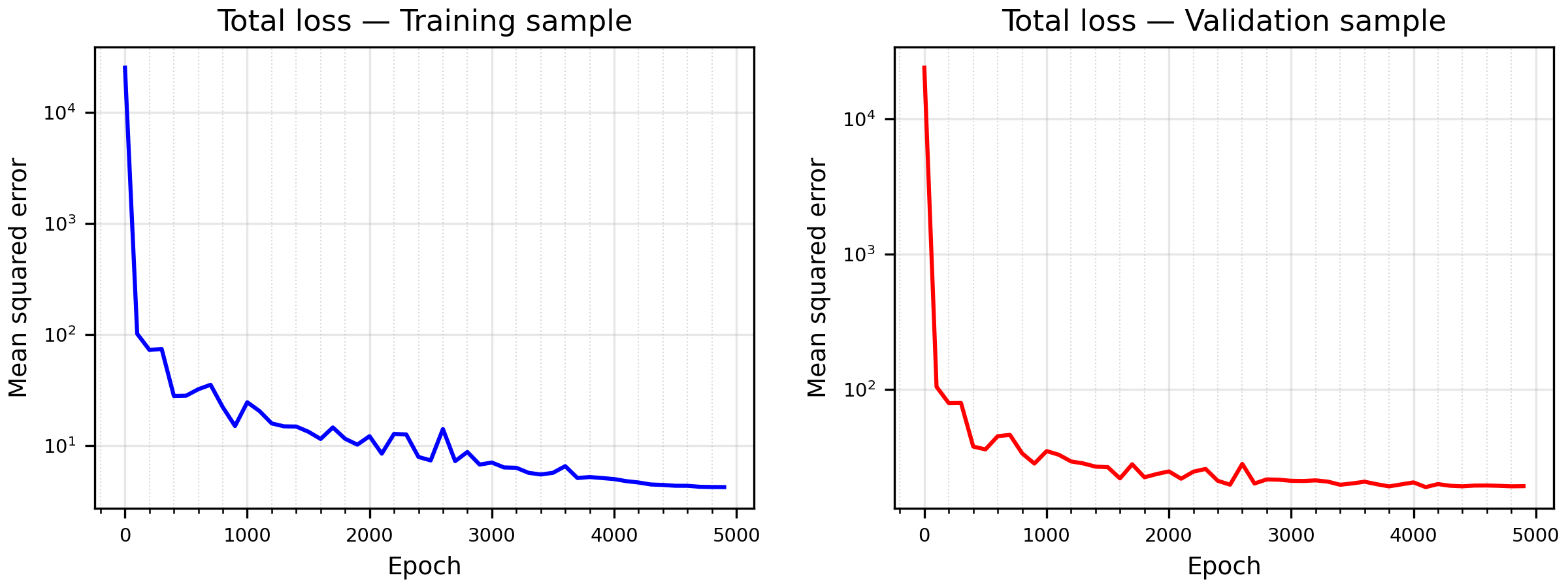
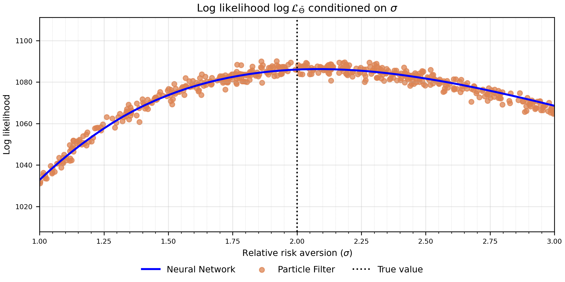
The script simulates 1,000 periods at the reference parameters and adds measurement error with a variance of 10% of each series’ variance. R is the measurement-error covariance. The particle filter then evaluates the log likelihood at 5,000 parameter vectors from a Sobol sequence, with 100 particles and 100 observations each. A second network with three hidden layers of 64 CELU units learns the map from parameters to log likelihood, holding out 20% of the draws for validation.

examples/rank/rank_baseline.py

data_path = folder / "observations.pt"
pf_dataset_path = folder / "datasets" / "likelihood.pt"
make_data = train_model or not data_path.exists()

if make_data:
    data = model.simulate(steps=1000, seed=12345)
    data, R = add_measurement_error(data, error_share=0.1, seed=12345)
    # Discard likelihood results that used the previous observations.
    pf_dataset_path.unlink(missing_ok=True)
    (folder / "surrogate.pt").unlink(missing_ok=True)
    (folder / "likelihood_sigma.pt").unlink(missing_ok=True)
    (folder / "likelihood_all.pt").unlink(missing_ok=True)
    torch.save({"data": data, "R": R}, data_path)
else:
    observations = torch.load(data_path, weights_only=True)
    data, R = observations["data"], observations["R"]

pf = ParticleFilter(model, data, R)

examples/rank/rank_baseline.py

surrogate_path = folder / "surrogate.pt"
train_pf_network = not load_pf_network or not load_pf_dataset or make_data or not surrogate_path.exists()
make_pf_dataset = train_pf_network and (not load_pf_dataset or make_data or not pf_dataset_path.exists())

if make_pf_dataset:
    print("Generating likelihood targets...")
    pf.generate_likelihood_dataset(
        N=5000, P=100, sim=100, burn=100, sobol=True, device=DEVICE, seed=12345,
    )
    pf_dataset_path.parent.mkdir(parents=True, exist_ok=True)
    torch.save(pf.dataset, pf_dataset_path)
elif train_pf_network:
    print("Loading the saved likelihood targets.")
    pf.dataset = torch.load(pf_dataset_path, weights_only=True)

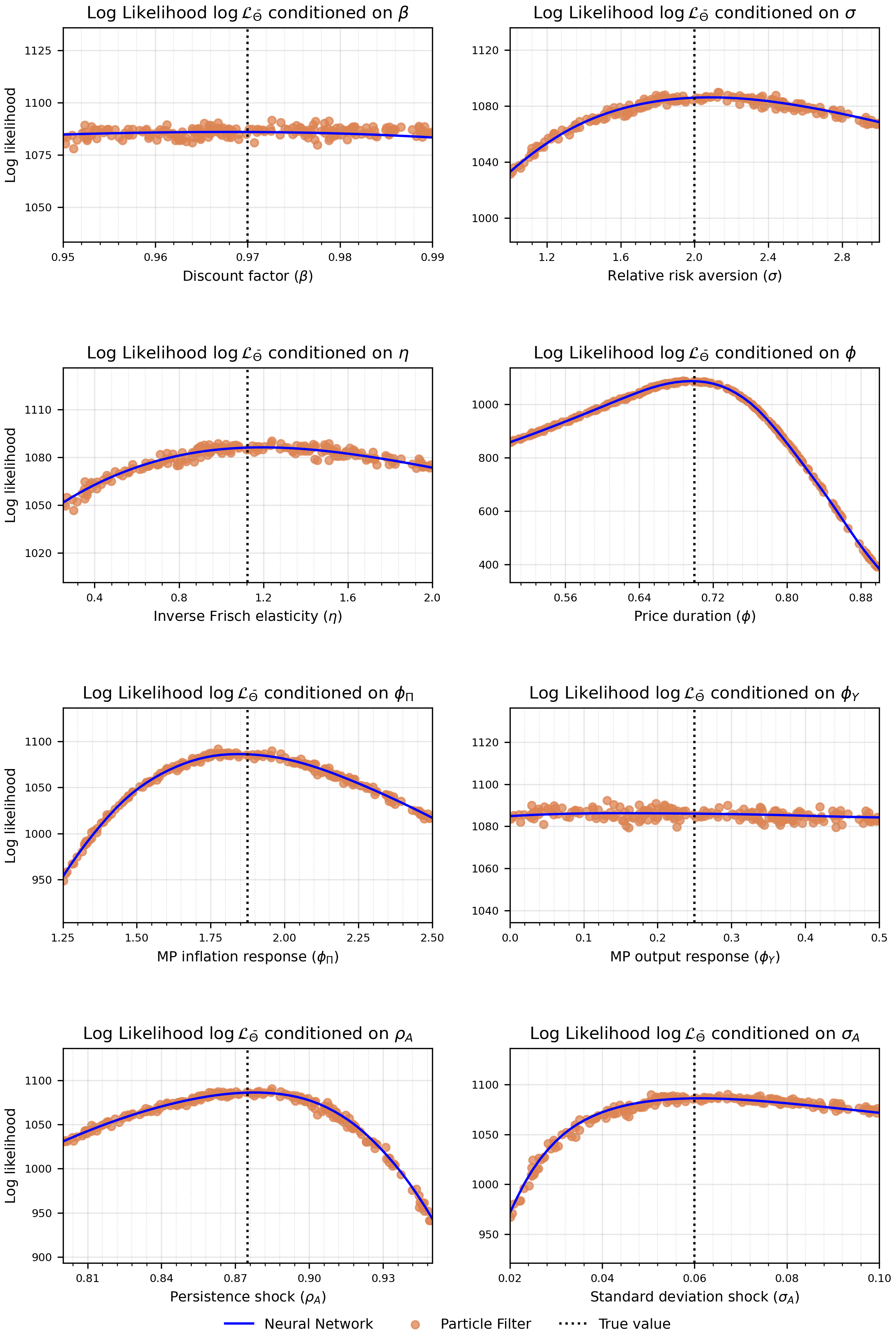
As in the paper, the notebook then varies one parameter at a time. It compares the network’s likelihood curve with particle-filter evaluations at random parameter values, first for risk aversion and then for every estimated parameter. These cells illustrate likelihood approximation. They do not return parameter estimates.

examples/rank/rank_baseline.py

if train_pf_network:
    (folder / "likelihood_sigma.pt").unlink(missing_ok=True)
    (folder / "likelihood_all.pt").unlink(missing_ok=True)
    print("Training the likelihood network...")
    pf.make_surrogate_network(hidden=64, layers=3, activation="CELU", seed=1234)
    pf.train(
        batch=100, epochs=5000, lr=1e-3, eta_min=1e-8,
        validation_share=0.2, print_after=100, device=DEVICE, seed=1234,
    )
    pf.dataset = None  # Targets are stored separately in pf_dataset_path.
    pf.save(folder, name="surrogate")
else:
    print("Loading the saved likelihood network.")
    pf.load(surrogate_path)

examples/rank/rank_baseline.py

likelihood_path = folder / "likelihood_sigma.pt"
likelihood_all_path = folder / "likelihood_all.pt"
# Use the same particle-filter settings as for the likelihood targets.
pf_settings = dict(P=100, sim=100, burn=100, seed=1234)

if train_pf_network or not likelihood_path.exists():
    likelihood = compute_likelihood(pf, "sigma", kind="surrogate", n=50)
    likelihood.update(compute_likelihood(pf, "sigma", kind="random", n=500, **pf_settings))
    torch.save(likelihood, likelihood_path)
else:
    likelihood = torch.load(likelihood_path, weights_only=True)

fig, _ = plot_posterior_single(
    likelihood, "sigma", true_value=model.par.sigma.item(), par_labels=parameter_labels,
)
save_figure(fig, str(figures / "likelihood"), format_list=["pdf", "png"])

Results

Training and validation mean squared error of the likelihood network.

Log likelihood as risk aversion \(\sigma\) varies, the other parameters at reference values. The line is the likelihood network and the dots are particle-filter evaluations at random values.

The same comparison for every estimated parameter.