Extension 7: Transforming observations
Observed series often use different units from the variables in the solved model.
Model
So far, we have used variables that we have already defined to solve the model. At the same time, estimation usually requires transforming the model variables to match them to the actual observed data. As a next step, we keep the economy of Extension 6 and modify our code to incorporate the following observation equation, which expresses the output gap in percent and annualizes quarterly inflation and interest-rate deviations,
\[ \begin{bmatrix}\text{Output gap}\\\text{Inflation}\\\text{Interest rate}\end{bmatrix} =\begin{bmatrix}100\hat X_t\\400\hat\Pi_t\\400\hat I_t\end{bmatrix}+u_t, \qquad u_t\sim N(0,\Sigma_u). \]
We also increase the measurement error so that \(m_E=0.25\) of each transformed series’ variance.
Neural network solution
Formulation
The policy network still returns deviations in model units. We change the units only in the observation equation, and the equilibrium residuals keep their original scale.
The loss is unchanged from Extension 1. It is the weighted mean of the squared residuals \(F_1\) (Euler equation), \(F_2\) (Phillips curve), and \(F_3\) (Taylor rule), with expectations approximated by Monte Carlo shock draws.
In the code
Transform before adding measurement error
We multiply output by 100 and inflation and the interest rate by 400. Then we collect these values in the observation dictionary.
examples/rank/rank_extension_07.py
def observe(self, obs_raw):
    # New in Extension 7: output gap in percent, inflation and the interest rate annualized.
return {"X": 100 * obs_raw["X"], "Pi": 400 * obs_raw["Pi"], "I": 400 * obs_raw["I"]}simulate returns these transformed observations. The notebook then adds measurement error with error_share=0.25. The particle filter applies exactly the same transformation to its predictions before comparing them with the data.
Results
Solution
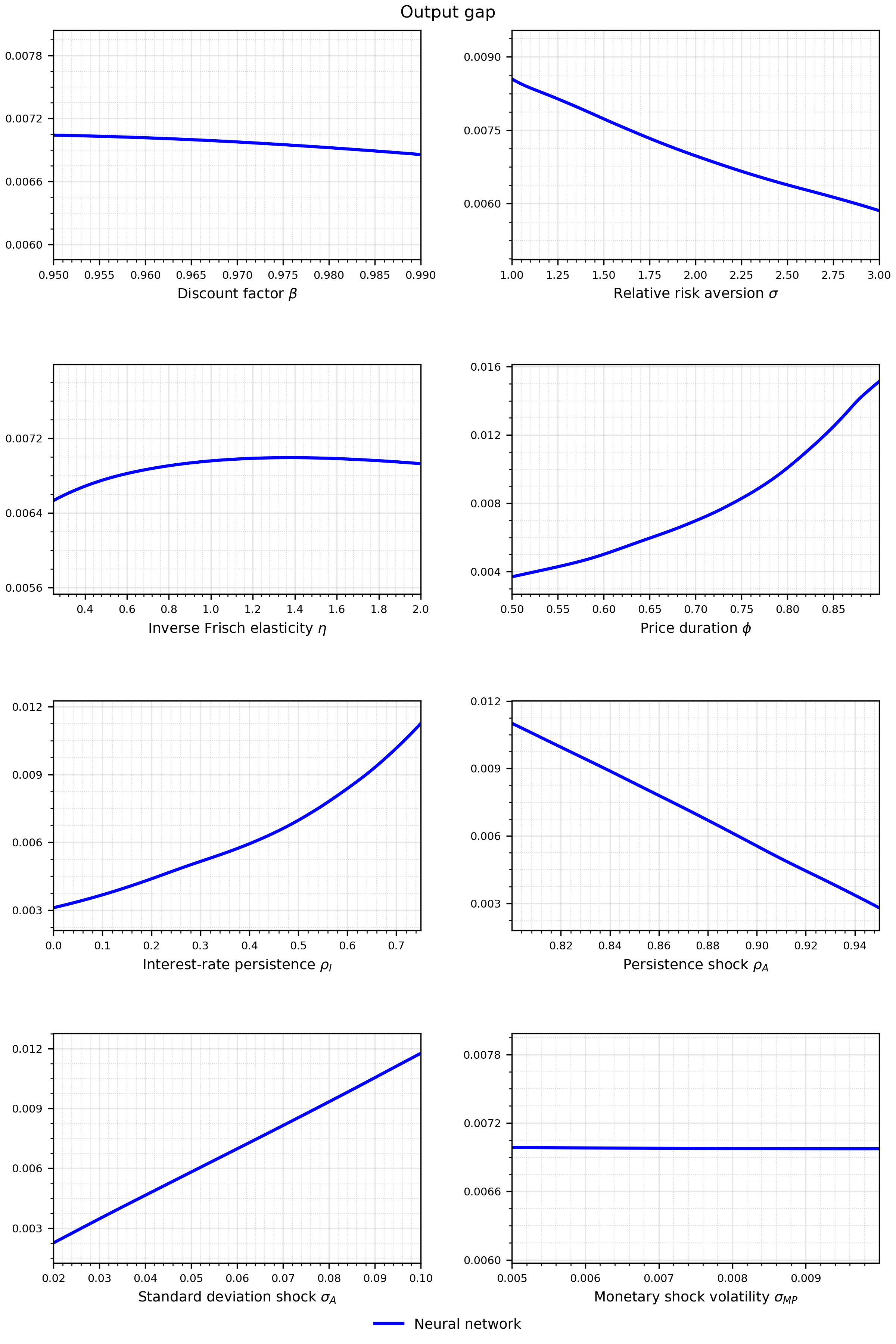
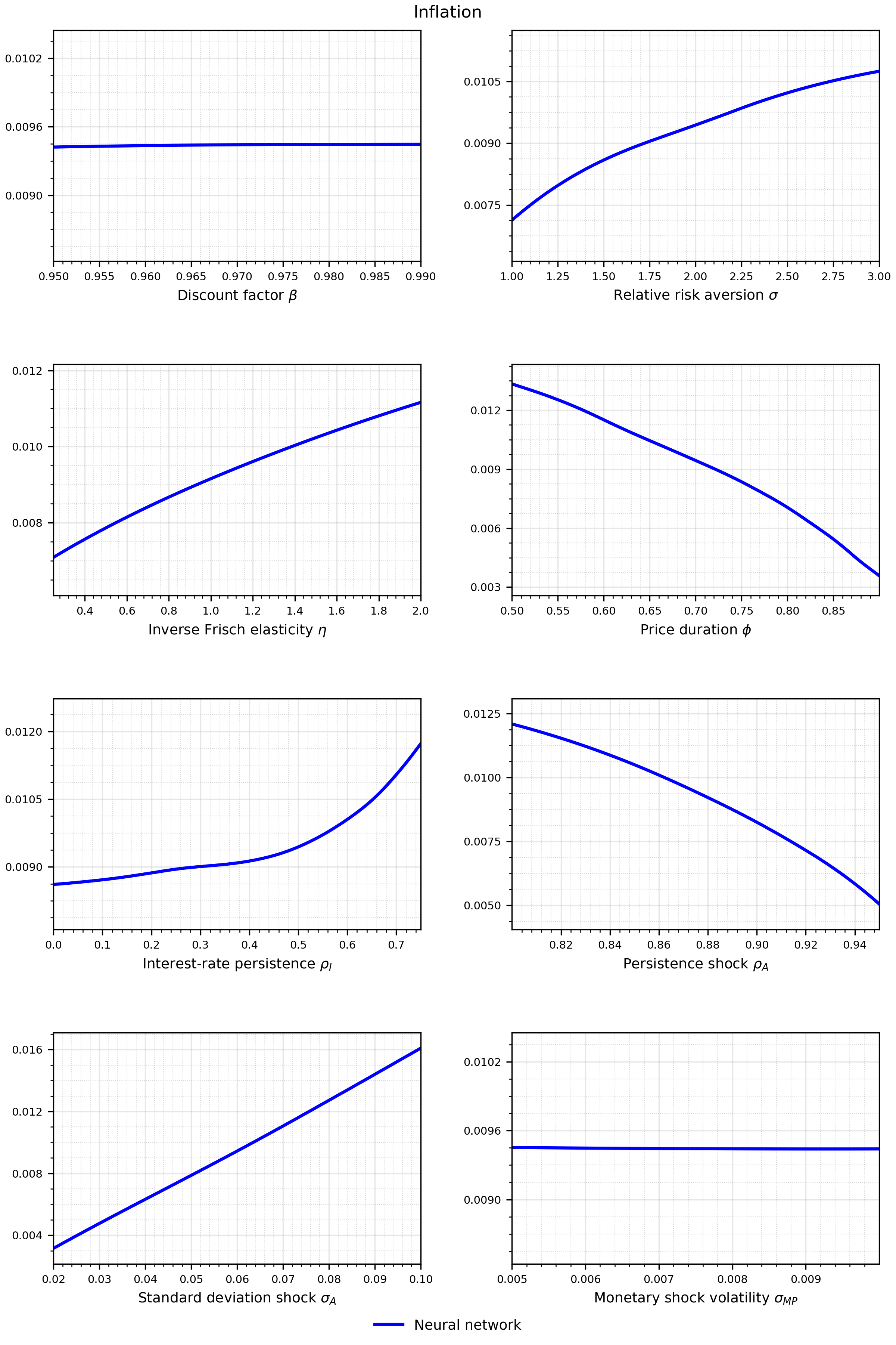
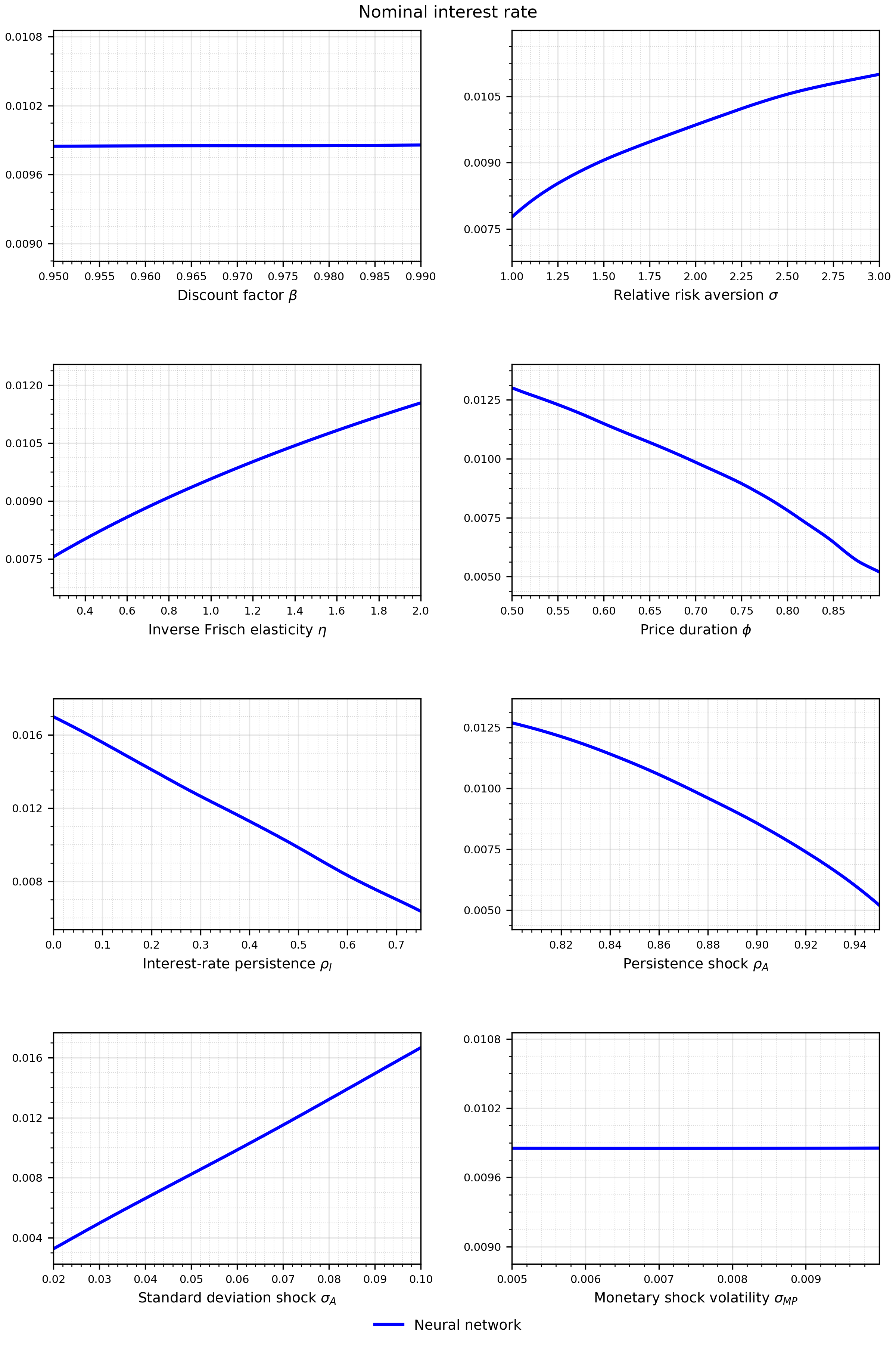
Likelihood