Extension 3: Endogenous state variables
We add the lagged nominal interest rate to the Taylor rule. This introduces an endogenous state variable.
Model
\[ \begin{aligned} \hat X_t &= E_t\hat X_{t+1}-\sigma^{-1}\left(\hat I_t-E_t\hat\Pi_{t+1}-\hat R_t^*\right),\\ \hat\Pi_t &= \kappa\hat X_t+\beta E_t\hat\Pi_{t+1},\\ \hat I_t &= \rho_I\hat I_{t-1}+(1-\rho_I)\left(\phi_\Pi\hat\Pi_t+\phi_Y\hat X_t\right),\\ \hat R_t^* &= \rho_A\hat R_{t-1}^*+\sigma(\rho_A-1)\omega\sigma_A\epsilon_t^A. \end{aligned} \]
We set the reference value of \(\rho_I\) to 0.5 and its bounds to 0 and 0.75.
Neural network solution
Formulation
The state now includes the lagged interest rate,
\[ \mathbb S_t=\{\hat R_t^*,\hat I_{t-1}\}. \]
The shocks, parameter sets, and policy outputs are unchanged.
In the code
Add a state and carry it into the next period
The lagged interest rate is named IL. It joins zeta in STATE_NAMES and therefore in the network inputs, with its own normalization bounds in state_bounds. initialize_state starts the simulated economies with lagged rates between \(-0.01\) and \(0.01\). The parameter list changes the reference value and range of rho_i.
next_state works as in the baseline but now also returns the lagged rate. First, compute next period’s natural rate from its exogenous transition equation. Then evaluate today’s policies at the current natural rate and lagged interest rate. The predicted I becomes next period’s IL, and expand_as repeats it across the shock draws so it has the same dimensions as zeta_next.
examples/rank/rank_extension_03.py
# New in Extension 3: the lagged interest rate is a state.
STATE_NAMES = ("zeta", "IL")

def state_bounds(self):
    return torch.tensor([-0.025, -0.025]), torch.tensor([0.025, 0.025])

def initialize_state(self, par=None, batch=100, device="cpu"):
    """Draw the natural rate from its stationary distribution."""
    par = self.par_draw if par is None else par
    loading = par.sigma_a * par.sigma * (par.rho_a - 1) * self.steady_state(par).omega
    std = ergodic_sigma(par.rho_a, loading.abs())
    # New in Extension 3: start with a range of lagged interest rates.
    lagged_rate = -0.01 + 0.02 * torch.rand(batch, 1, device=device)
    zeta = torch.randn(batch, 1, device=device) * std
    return State({"zeta": zeta, "IL": lagged_rate})

@torch.no_grad()
def next_state(self, e):
    """Return next period's state for the shock draws in e, without changing the current state."""
    par = self.par_draw
    loading = par.sigma_a * par.sigma * (par.rho_a - 1) * self.ss.omega
    zeta_next = par.rho_a * self.state.zeta + loading * e.zeta
    # New in Extension 3: today's interest rate becomes next period's lagged rate.
    # Repeat it across the shock draws to match the shape of zeta_next.
    _, _, I = self.policy()
return State({"zeta": zeta_next, "IL": I.expand_as(zeta_next)})The returned State contains both next-period variables, zeta and IL. Today’s state remains unchanged. The residual calculation below uses this returned state to evaluate future policies and form expectations.
Include the lagged rate in the Taylor rule
Finally, we add \(\rho_I\hat I_{t-1}\) to the Taylor rule. The full residual calculation below shows how the new state enters the equation, with a comment marking the addition.
examples/rank/rank_extension_03.py
def residuals(self, e, detach_next=True):
    par = self.par_draw

    # Evaluate today's policies.
    X, Pi, I = self.policy()

    # Next period's state for each shock draw.
    state_next = self.next_state(e)

    # Evaluate next period's policies at that state.
    with torch.set_grad_enabled(not detach_next):
        X_next, Pi_next, _ = self.policy(state_next)

    # Average over the draws to approximate the conditional expectations.
    EX_next = X_next.mean(dim=0)
    EPi_next = Pi_next.mean(dim=0)

    # F_1: Euler equation.
    euler = X - (EX_next - (I - EPi_next - self.state.zeta) / par.sigma)
    # F_2: Phillips curve.
    phillips = Pi - (self.ss.kappa * X + par.beta * EPi_next)
    # F_3: Taylor rule. New in Extension 3: the lagged interest rate enters.
    taylor = I - (par.rho_i * self.state.IL + (1 - par.rho_i) * (par.phipi * Pi + par.phiy * X))
return [euler, phillips, taylor]Results
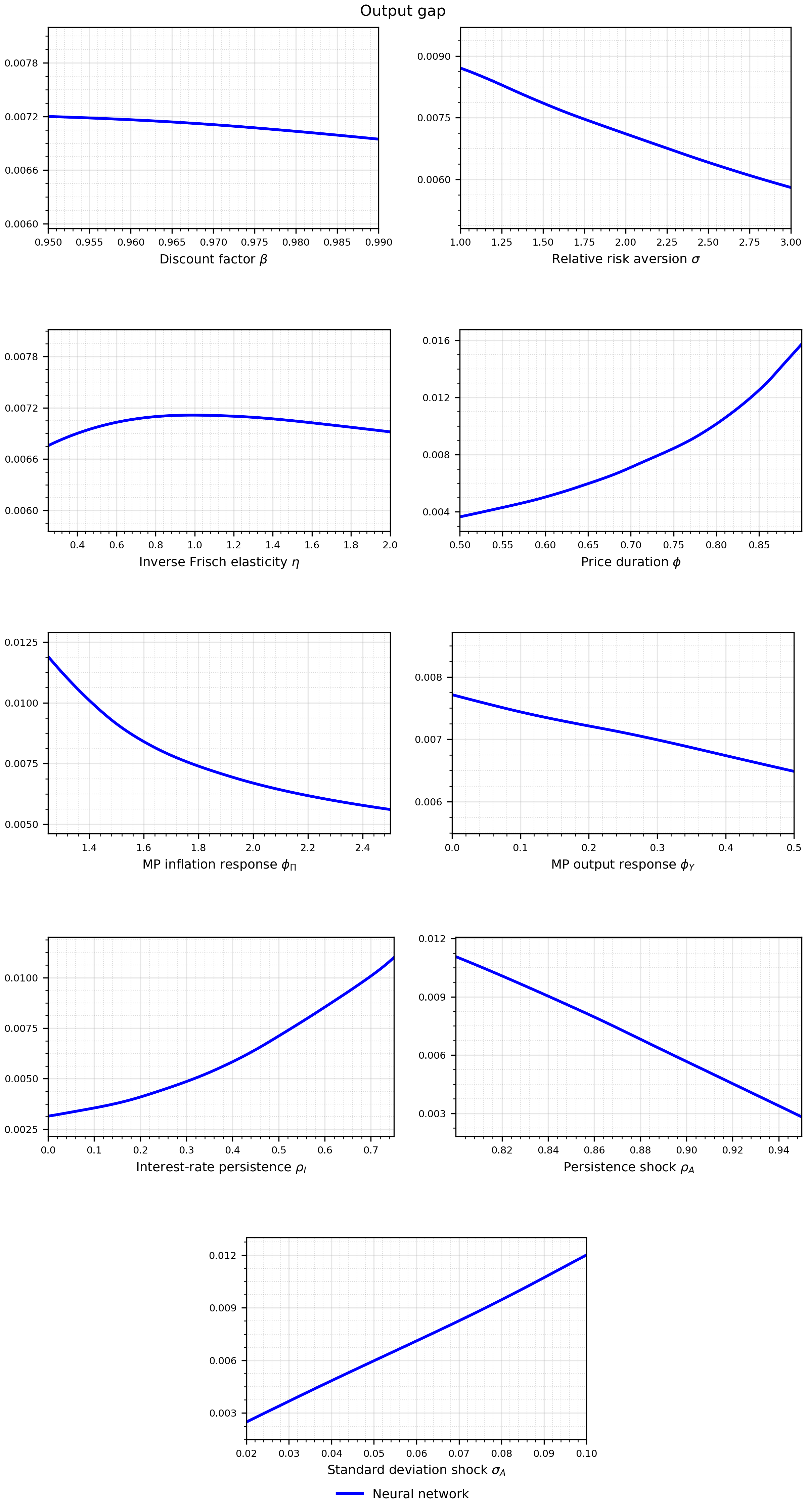
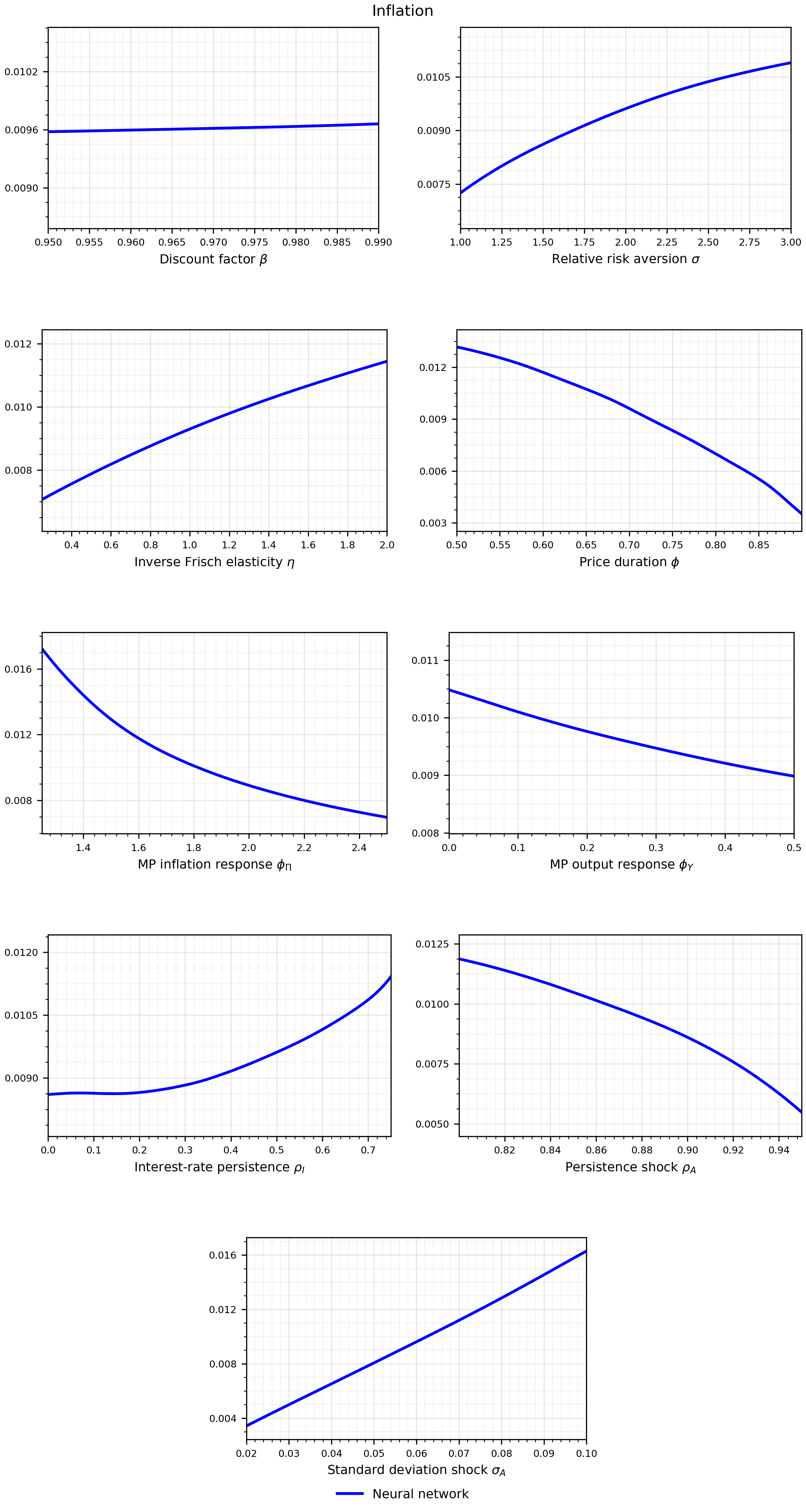
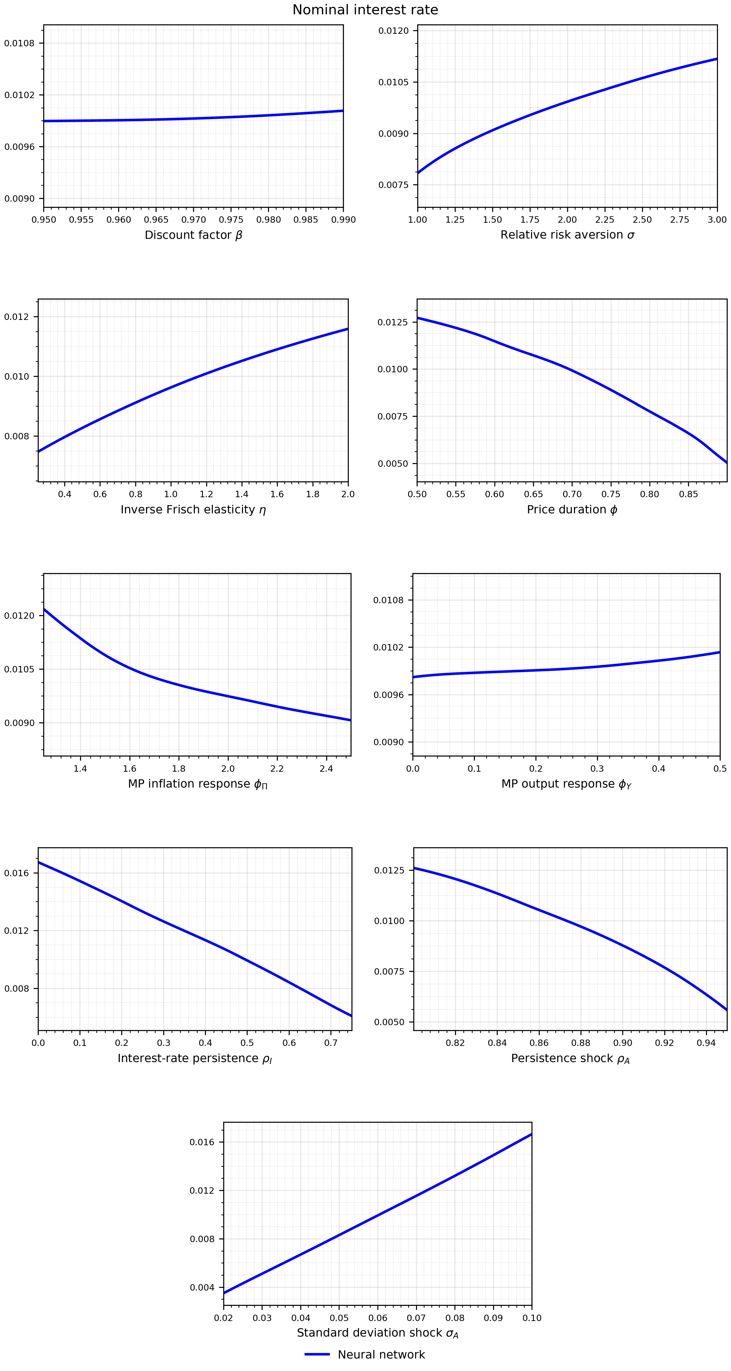
Solution
Likelihood