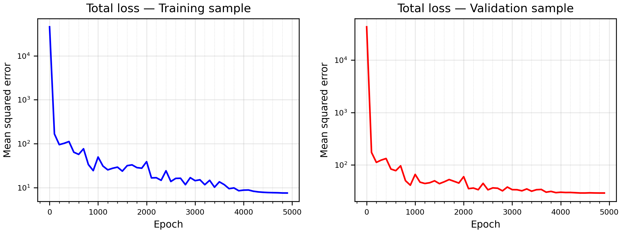
Extension 1: Policy functions
We add the nominal interest rate as a policy function. The Taylor rule becomes a separate equation, instead of being substituted into the Euler equation.
Model
\[ \begin{aligned} \hat X_t &= E_t\hat X_{t+1}-\sigma^{-1}\left(\hat I_t-E_t\hat\Pi_{t+1}-\hat R_t^*\right),\\ \hat\Pi_t &= \kappa\hat X_t+\beta E_t\hat\Pi_{t+1},\\ \hat I_t &= \phi_\Pi\hat\Pi_t+\phi_Y\hat X_t,\\ \hat R_t^* &= \rho_A\hat R_{t-1}^*+\sigma(\rho_A-1)\omega\sigma_A\epsilon_t^A. \end{aligned} \]
Neural network solution
Formulation
The network now also learns the nominal interest rate,
\[ \begin{pmatrix}\hat X_t\\\hat\Pi_t\\\hat I_t\end{pmatrix} =\psi_{NN}(\mathbb S_t,\tilde\Theta\mid\bar\Theta). \]
The Taylor rule joins the equations whose errors are minimized,
\[ \begin{aligned} F_1 &= \hat X_t-\left[E_t\hat X_{t+1} -\sigma^{-1}\left(\hat I_t-E_t\hat\Pi_{t+1}-\hat R_t^*\right)\right],\\ F_2 &= \hat\Pi_t-\left(\kappa\hat X_t+\beta E_t\hat\Pi_{t+1}\right),\\ F_3 &= \hat I_t-\left(\phi_\Pi\hat\Pi_t+\phi_Y\hat X_t\right). \end{aligned} \]
The state, shocks, and parameter sets are unchanged.
The loss is the weighted mean of the squared equation errors over a training batch,
\[ \mathcal L=\frac{1}{N_{batch}}\sum_{b=1}^{N_{batch}}\sum_{j=1}^{3}\alpha_j\left(F_j^{(b)}\right)^2. \]
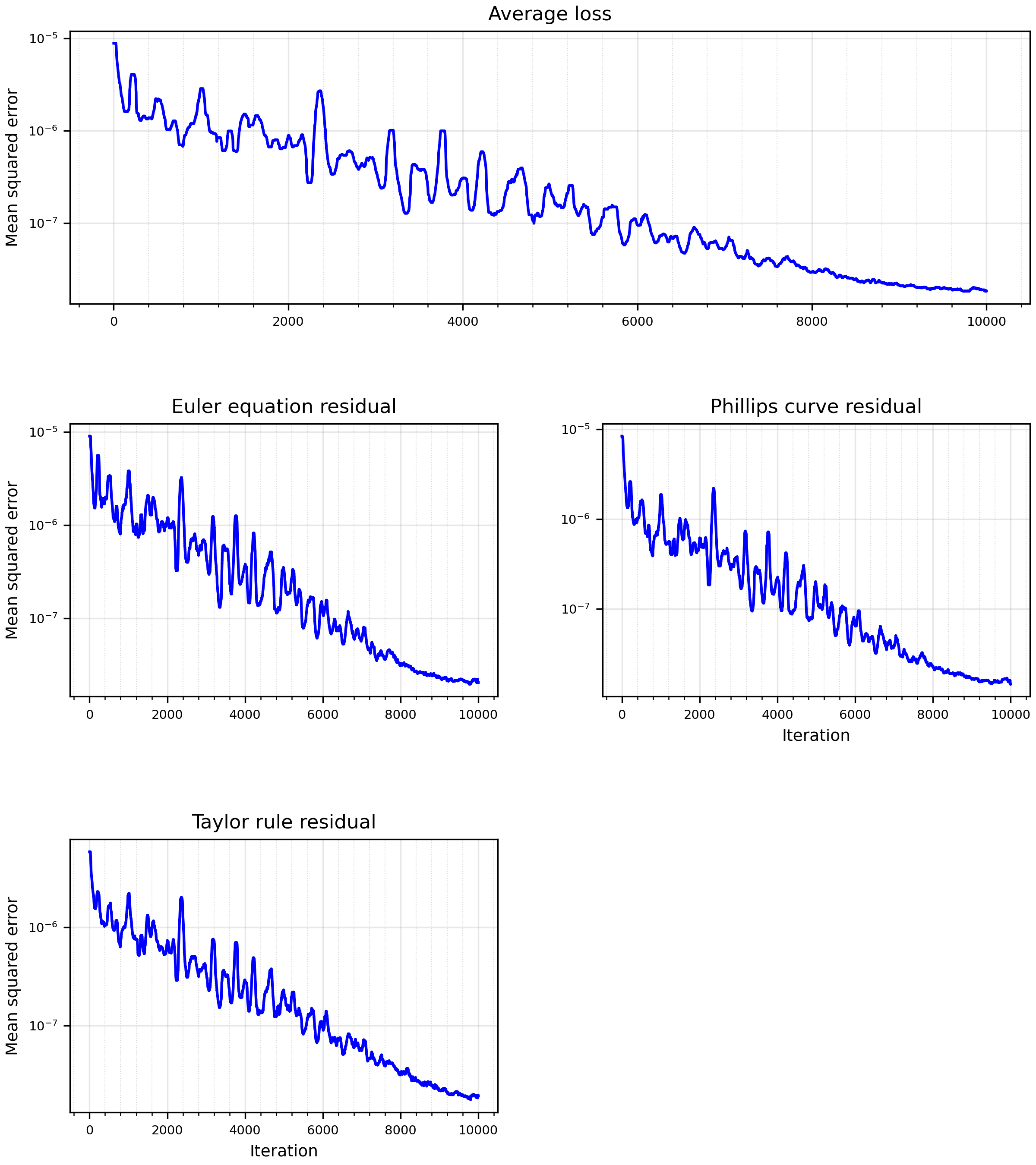
Here \(N_{batch}\) is the number of simulated economies in a training batch and \(F_j^{(b)}\) is equation \(j\)’s residual for economy \(b\). As in the baseline, every equation weight is \(\alpha_j=1000\).
In the code
Add the interest-rate output
The baseline network returned output and inflation. Adding I to POLICY_NAMES gives it a third output for the nominal interest rate. In policy, assign the third output column to I, divide each prediction by 100 as in the baseline, and return all three policies in model units. The notebook contains the complete model, including the network and training loop.
examples/rank/rank_extension_01.py
# New in Extension 1: the network also returns the nominal interest rate.
POLICY_NAMES = ("X", "Pi", "I")

def policy(self, state=None, par=None):
    state = self.state if state is None else state
    par = self.par_draw if par is None else par

    # Vectors of states and parameters.
    states = state.cat(keys=self.STATE_NAMES)
    parameters = par.cat()

    # Future states have an extra leading dimension for the shock draws.
    # Repeat the parameters along it to evaluate expectations.
    if states.dim() > parameters.dim():
        parameters = parameters.expand(states.shape[0], *parameters.shape)

    # Evaluate the network on the combined inputs.
    inputs = torch.cat((states, parameters), dim=-1)
    output = self.network(inputs)

    X = output[..., 0:1] / 100
    Pi = output[..., 1:2] / 100
    I = output[..., 2:3] / 100

return X, Pi, IAdjust the equation errors
As in the baseline, we evaluate current policies, simulate next-period states, and average future output and inflation over shocks. Two things change. The Euler equation uses the network’s I output directly, and a third residual measures its difference from the Taylor rule.
examples/rank/rank_extension_01.py
def residuals(self, e, detach_next=True):
    par = self.par_draw

    # Evaluate today's policies.
    X, Pi, I = self.policy()

    # Next period's state for each shock draw.
    state_next = self.next_state(e)

    # Evaluate next period's policies at that state.
    with torch.set_grad_enabled(not detach_next):
        X_next, Pi_next, _ = self.policy(state_next)

    # Average over the draws to approximate the conditional expectations.
    EX_next = X_next.mean(dim=0)
    EPi_next = Pi_next.mean(dim=0)

    # F_1: Euler equation.
    euler = X - (EX_next - (I - EPi_next - self.state.zeta) / par.sigma)
    # F_2: Phillips curve.
    phillips = Pi - (self.ss.kappa * X + par.beta * EPi_next)
    # New in Extension 1: F_3, the Taylor rule.
    taylor = I - (par.phipi * Pi + par.phiy * X)
return [euler, phillips, taylor]In TrainingConfig, weights=ConstantWeights([1000.0, 1000.0, 1000.0]) sets \(\alpha_1\), \(\alpha_2\), and \(\alpha_3\) in the residual order. Set load_model = False after changing the weights.
The nominal rate also becomes an observable
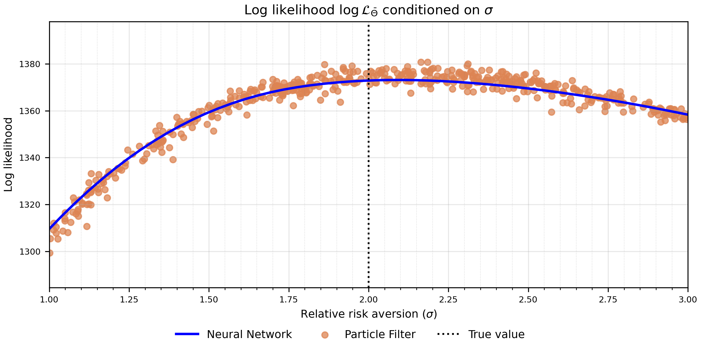
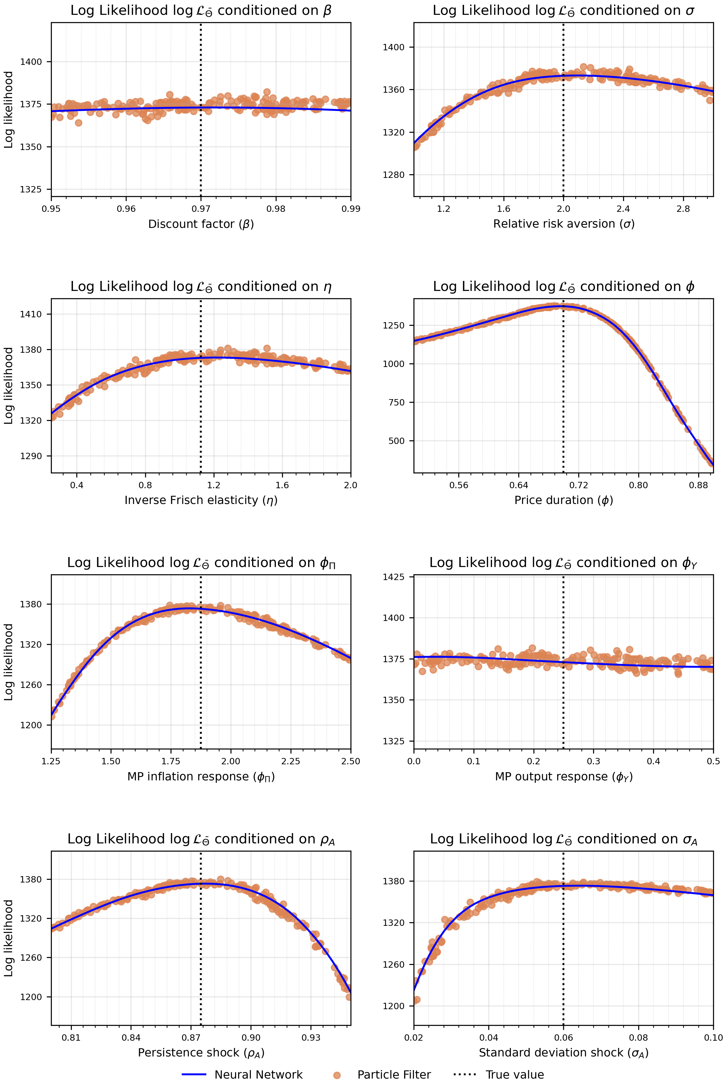
Until Extension 6, the observation equation contains every variable the model determines, which here is the natural rate and each policy output. Making \(\hat I_t\) a policy therefore adds it to the simulated data and to the particle filter’s observation equation. The economy is unchanged. Under this Taylor rule \(\hat I_t\) is an exact function of \(\hat\Pi_t\) and \(\hat X_t\), so the extra series is a second noisy signal of output and inflation. Because the data differ, the likelihood values are not comparable with the baseline’s. Extension 6 shows how to choose the observed variables explicitly.
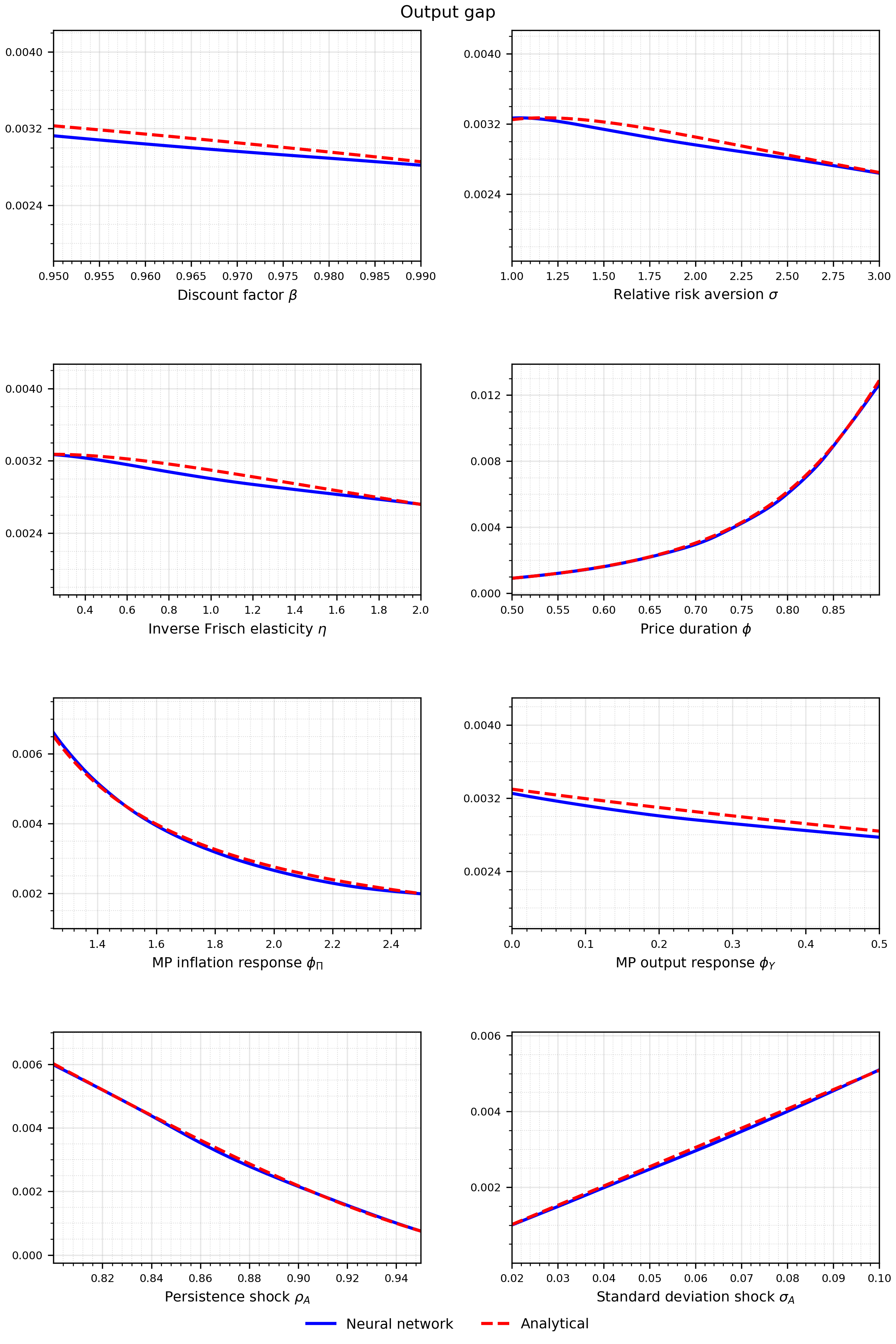
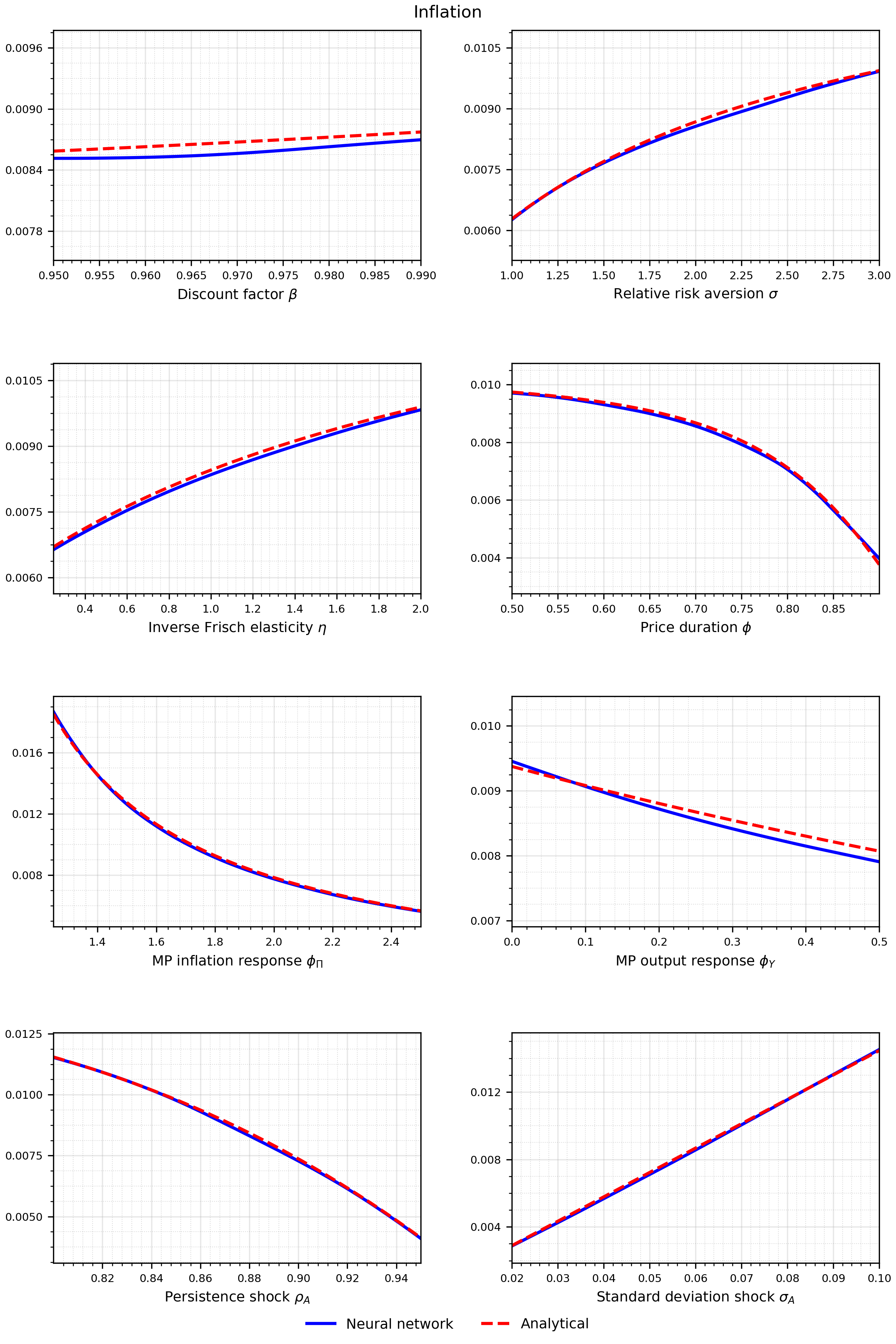
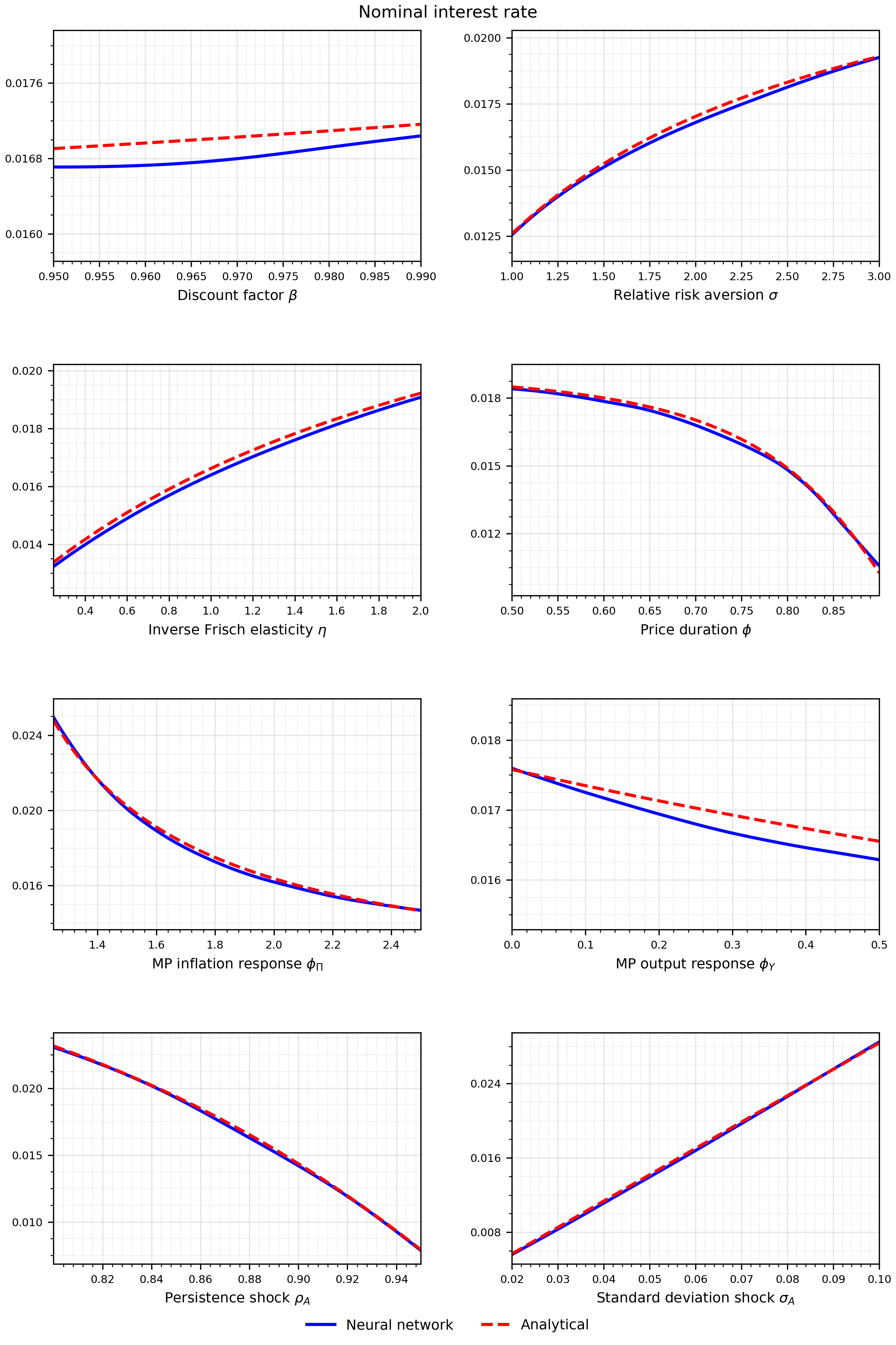
Results
Solution
Likelihood