Extension 5: Pseudo-state variables
We now fix two parameters and keep the others available for estimation.
Model
The economic equations and shocks are those of Extension 4. We now fix the Taylor-rule responses at \(\phi_\Pi=1.875\) and \(\phi_Y=0.25\).
Neural network solution
Formulation
The varying and calibrated parameter sets are
\[\tilde\Theta=\{\beta,\sigma,\eta,\phi,\rho_I,\rho_A,\sigma_A,\sigma_{MP}\},\qquad \bar\Theta=\{\phi_\Pi,\phi_Y\}.\]
The network takes the three states and eight varying parameters. The eight varying parameters are the pseudo-state variables. The calibrated coefficients still enter the model equations, but they are not network inputs and do not vary across training draws.
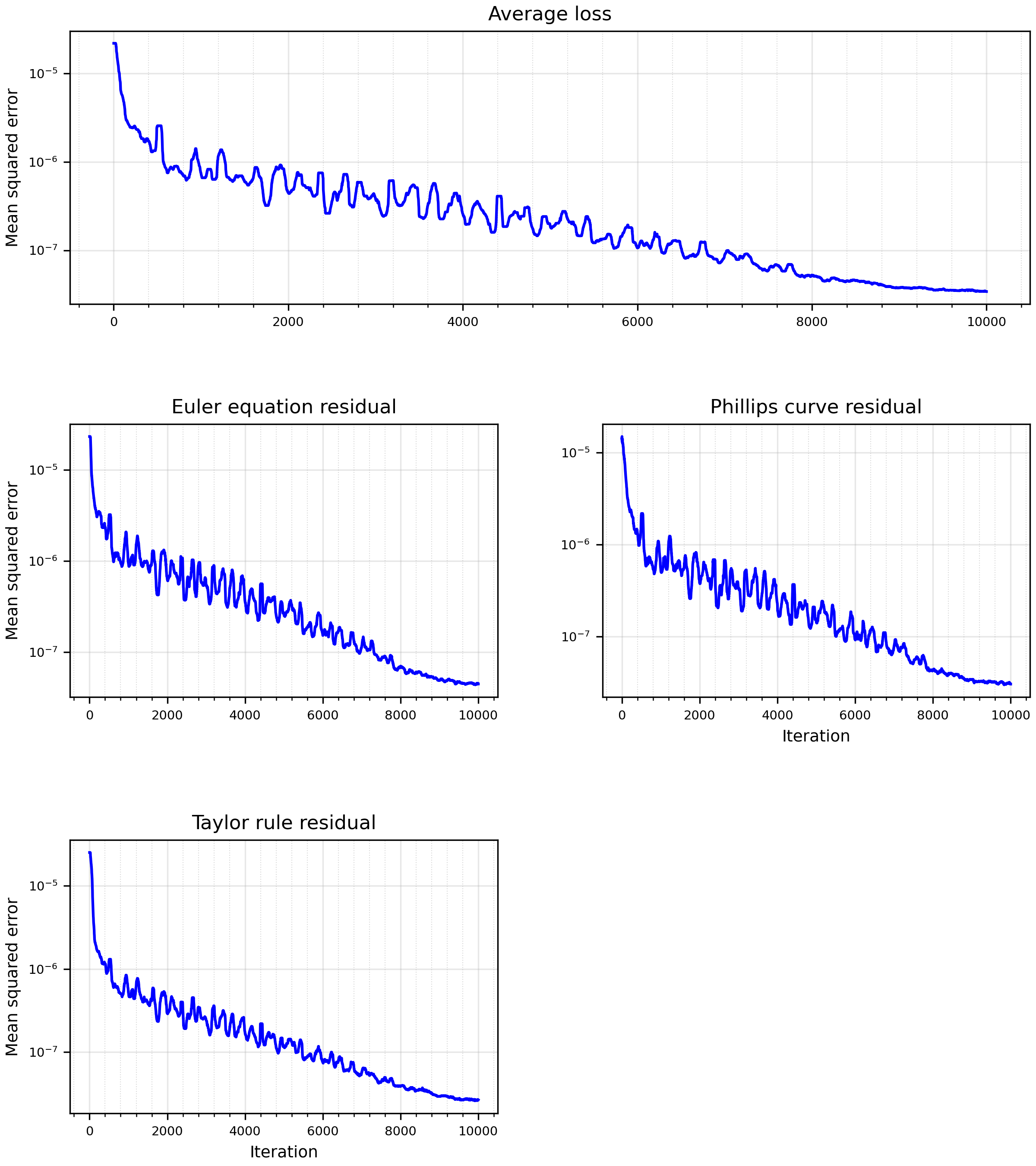
The loss is unchanged from Extension 1. It is the weighted mean of the squared residuals \(F_1\) (Euler equation), \(F_2\) (Phillips curve), and \(F_3\) (Taylor rule), with expectations approximated by Monte Carlo shock draws.
In the code
Specify values and sampling ranges
PARAMETERS gives the reference values of every parameter. RANGES contains only the parameters that vary. Omitting a parameter from RANGES fixes it at its reference value.
examples/rank/rank_extension_05.py
# Training ranges. Every parameter with a range is a network input.
# New in Extension 5: phipi and phiy have no range, so they stay at their reference values.
RANGES = {
    "beta": torch.distributions.Uniform(0.95, 0.99),
    "sigma": torch.distributions.Uniform(1.0, 3.0),
    "eta": torch.distributions.Uniform(0.25, 2.0),
    "phi": torch.distributions.Uniform(0.5, 0.9),
    "rho_i": torch.distributions.Uniform(0.0, 0.75),
    "rho_a": torch.distributions.Uniform(0.8, 0.95),
    "sigma_a": torch.distributions.Uniform(0.02, 0.1),
    "sigma_mp": torch.distributions.Uniform(0.005, 0.01),
}Build the network inputs
Ranges keeps the calibrated values fixed when drawing parameters for training, simulation, and filtering. ranges.keys_estimable lists the eight parameters that vary. make_network normalizes only these inputs, and policy passes only these parameters to the network. The likelihood interface keeps the full parameter vector, including the constants.
examples/rank/rank_extension_05.py
def make_network(self, hidden=64, layers=5, activation=torch.nn.CELU):
    """Normalize states and parameters, then apply a fully connected network."""
    layer_list = []

    # Normalize layer
    state_low, state_high = self.state_bounds()
    # New in Extension 5: only the parameters with a range are inputs.
    keys = self.ranges.keys_estimable()
    low = torch.cat((state_low, self.ranges.low_tensor(keys)))
    high = torch.cat((state_high, self.ranges.high_tensor(keys)))
    layer_list.append(NormalizeLayer(low, high))

    # First layer
    layer_list.append(torch.nn.Linear(len(low), hidden))
    layer_list.append(activation())

    # Middle layers
    for _ in range(1, layers):
        layer_list.append(torch.nn.Linear(hidden, hidden))
        layer_list.append(activation())

    # Last layer
    layer_list.append(torch.nn.Linear(hidden, len(self.POLICY_NAMES)))

    return torch.nn.Sequential(*layer_list)
examples/rank/rank_extension_05.py
def policy(self, state=None, par=None):
    state = self.state if state is None else state
    par = self.par_draw if par is None else par

    # Vectors of states and parameters.
    states = state.cat(keys=self.STATE_NAMES)
    # New in Extension 5: pass only the parameters with a range.
    parameters = par.cat(keys=self.ranges.keys_estimable())

    # Future states have an extra leading dimension for the shock draws.
    # Repeat the parameters along it to evaluate expectations.
    if states.dim() > parameters.dim():
        parameters = parameters.expand(states.shape[0], *parameters.shape)

    # Evaluate the network on the combined inputs.
    inputs = torch.cat((states, parameters), dim=-1)
    output = self.network(inputs)

    X = output[..., 0:1] / 100
    Pi = output[..., 1:2] / 100
    I = output[..., 2:3] / 100

return X, Pi, IResults
Solution
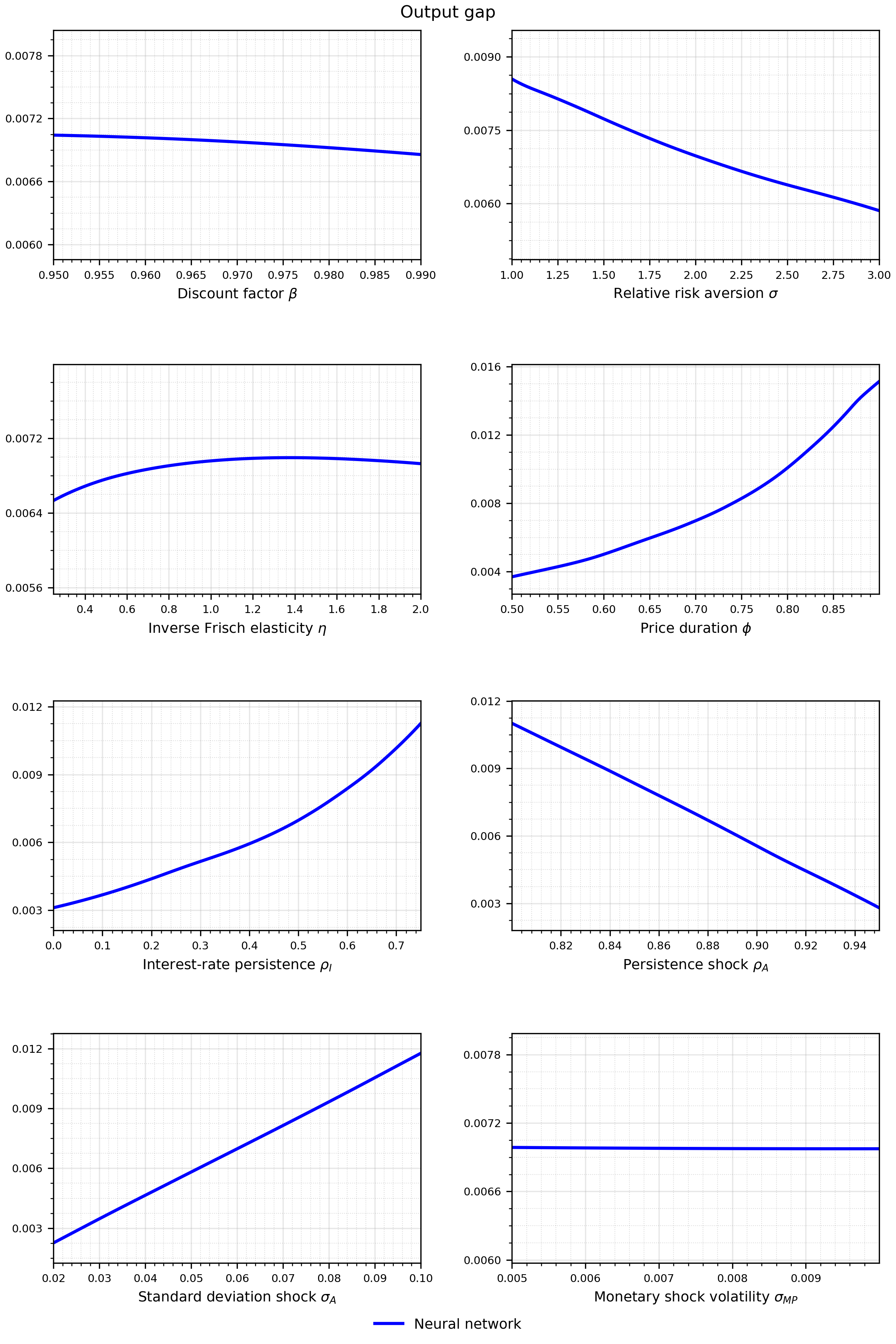
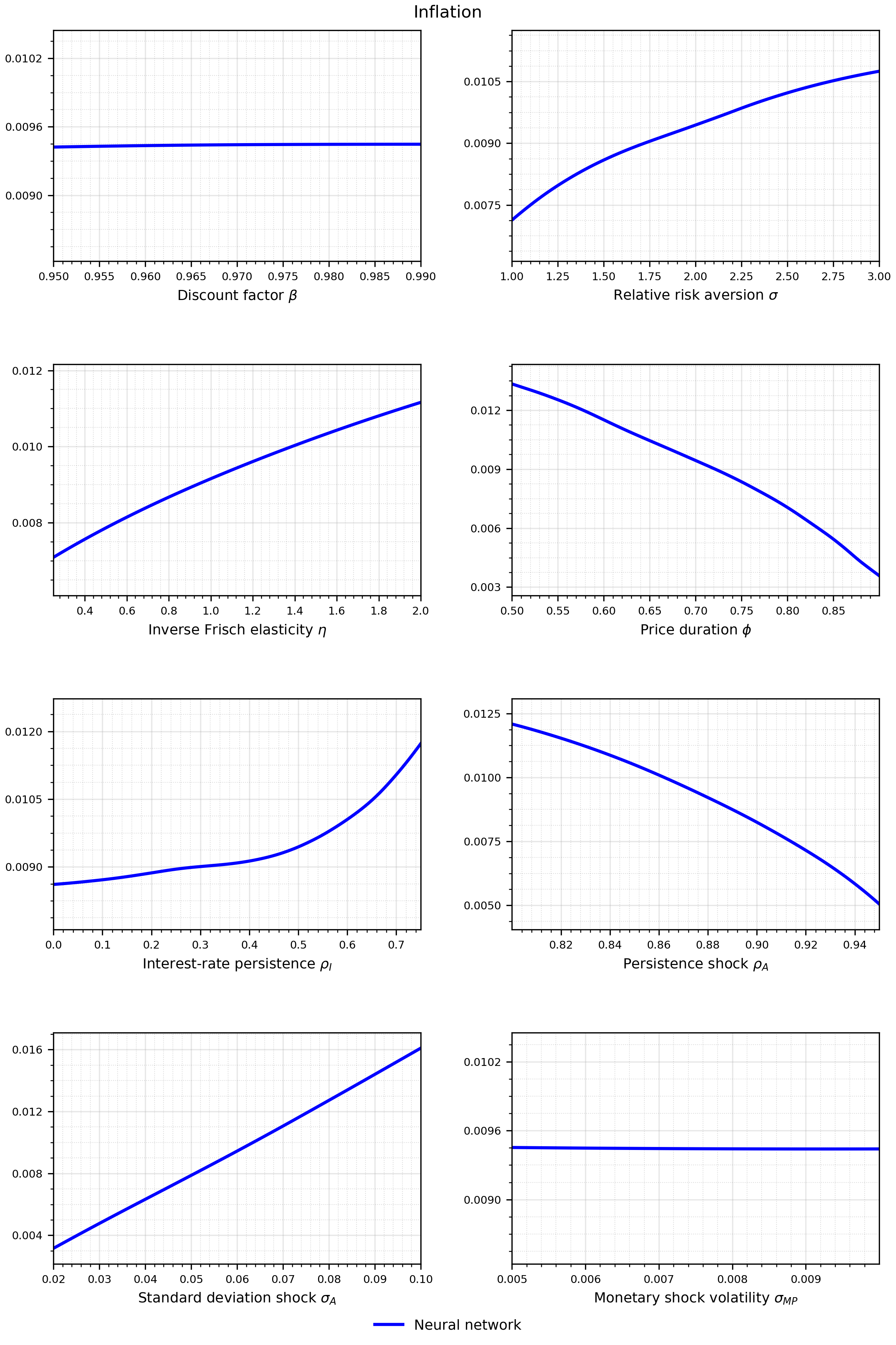
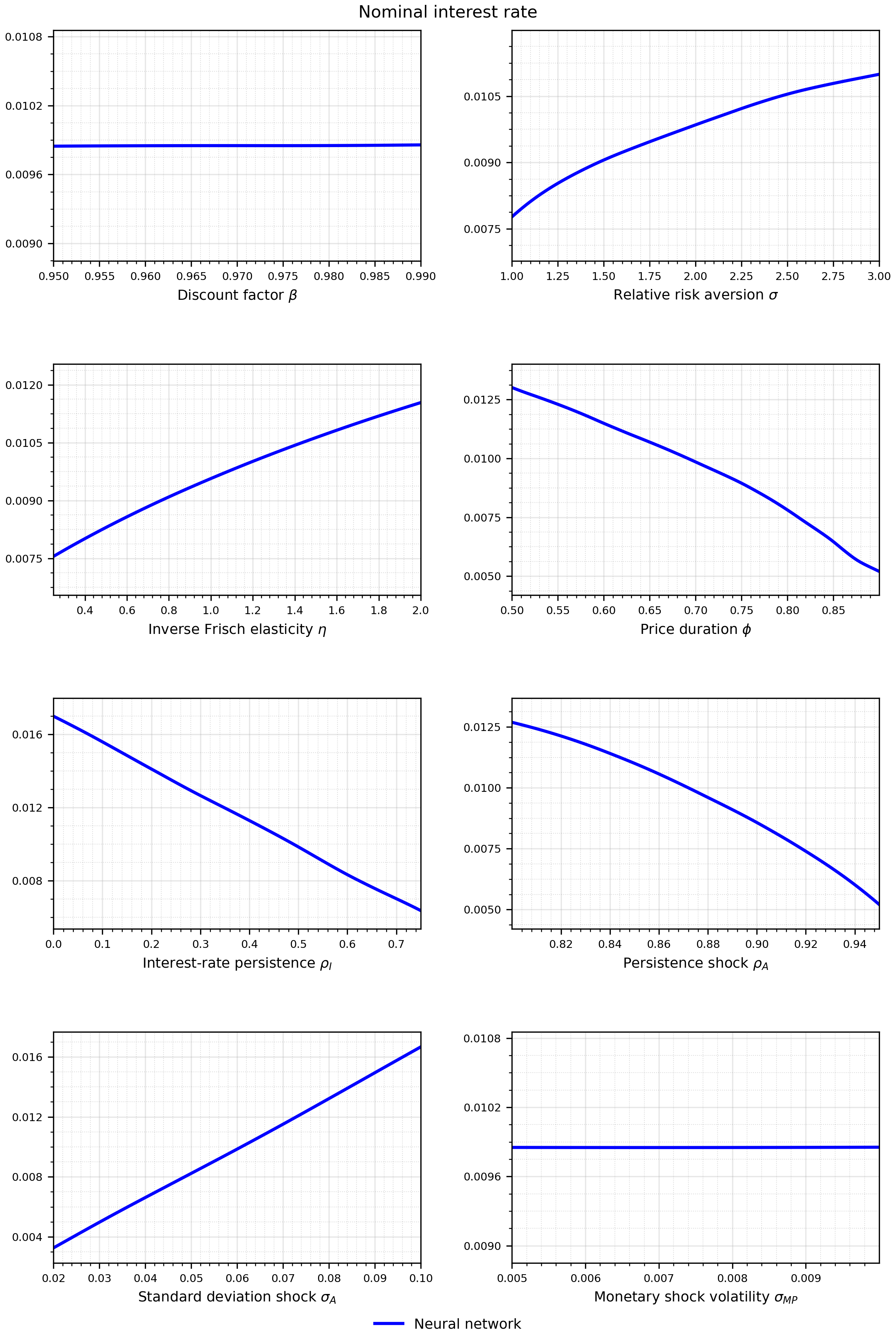
Likelihood