Extension 4: Shocks and exogenous states
We add a monetary-policy shock to the Taylor rule.
Model
The economy has an output gap \(\hat X_t\), inflation \(\hat\Pi_t\), and a nominal rate \(\hat I_t\),
\[ \begin{aligned} \hat X_t&=E_t\hat X_{t+1}-\sigma^{-1}(\hat I_t-E_t\hat\Pi_{t+1}-\hat R_t^*),\\ \hat\Pi_t&=\kappa\hat X_t+\beta E_t\hat\Pi_{t+1},\\ \hat I_t&=\rho_I\hat I_{t-1}+(1-\rho_I)(\phi_\Pi\hat\Pi_t+\phi_Y\hat X_t)+\widehat{mp}_t,\\ \hat R_t^*&=\rho_A\hat R_{t-1}^*+\sigma(\rho_A-1)\omega\sigma_A\epsilon_t^A,\\ \widehat{mp}_t&=\sigma_{MP}\epsilon_t^{MP}. \end{aligned} \]
Here \(\kappa=(1-\phi)(1-\phi\beta)(\sigma+\eta)/\phi\) and \(\omega=(1+\eta)/(\sigma+\eta)\). Both innovations \(\epsilon_t^A\) and \(\epsilon_t^{MP}\) are independent and standard normal. The monetary-shock volatility \(\sigma_{MP}\) is a new parameter with reference value 0.0075 and training range \([0.005, 0.01]\).
Neural network solution
Formulation
The state, shocks, and estimated parameters are
\[ \mathbb S_t=\{\hat R_t^*,\hat I_{t-1},\widehat{mp}_t\},\qquad \nu_t=\{\epsilon_t^A,\epsilon_t^{MP}\},\qquad \tilde\Theta=\{\beta,\sigma,\eta,\phi,\phi_\Pi,\phi_Y,\rho_I,\rho_A,\sigma_A,\sigma_{MP}\}. \]
The network returns all three policies \((\hat X_t,\hat\Pi_t,\hat I_t)\). We draw both shocks when calculating expectations. The lagged rate is still determined by today’s interest-rate policy. The monetary shock is also added to the observations.
The loss is unchanged from Extension 1. It is the weighted mean of the squared residuals \(F_1\) (Euler equation), \(F_2\) (Phillips curve), and \(F_3\) (Taylor rule), with expectations approximated by Monte Carlo shock draws.
In the code
Add the monetary shock and its volatility
sigma_mp joins the parameters, after the productivity-shock parameters. Its training range adds one more parameter input to the network. SHOCKS adds a standard-normal monetary innovation, which the model scales by its volatility.
examples/rank/rank_extension_04.py
# Reference values. They also generate the data later on.
PARAMETERS = {
    "beta": 0.97,
    "sigma": 2.0,
    "eta": 1.125,
    "phi": 0.7,
    "phipi": 1.875,
    "phiy": 0.25,
    "rho_i": 0.5,  # New in Extension 3: positive reference value.
    "rho_a": 0.875,
    "sigma_a": 0.06,
    "sigma_mp": 0.0075,  # New in Extension 4: monetary-shock volatility.
}

# Training ranges. Every parameter with a range is a network input.
RANGES = {
    "beta": torch.distributions.Uniform(0.95, 0.99),
    "sigma": torch.distributions.Uniform(1.0, 3.0),
    "eta": torch.distributions.Uniform(0.25, 2.0),
    "phi": torch.distributions.Uniform(0.5, 0.9),
    "phipi": torch.distributions.Uniform(1.25, 2.5),
    "phiy": torch.distributions.Uniform(0.0, 0.5),
    "rho_i": torch.distributions.Uniform(0.0, 0.75),
    "rho_a": torch.distributions.Uniform(0.8, 0.95),
    "sigma_a": torch.distributions.Uniform(0.02, 0.1),
    "sigma_mp": torch.distributions.Uniform(0.005, 0.01),
}

# Distributions of the shock innovations.
SHOCKS = {"zeta": torch.distributions.Normal(0.0, 1.0), "mp": torch.distributions.Normal(0.0, 1.0)}Advance the state
mp joins the states. initialize_state draws today’s monetary shock, and next_state uses each shock draw to form tomorrow’s natural rate and monetary shock, scaling the monetary innovation by sigma_mp. Today’s predicted interest rate becomes tomorrow’s lagged rate. The returned state has one entry for each Monte Carlo draw, economy, and state variable.
examples/rank/rank_extension_04.py
# New in Extension 3: the lagged interest rate is a state.
# New in Extension 4: the monetary shock is an exogenous state.
STATE_NAMES = ("zeta", "IL", "mp")

def initialize_state(self, par=None, batch=100, device="cpu"):
    """Draw the natural rate from its stationary distribution."""
    par = self.par_draw if par is None else par
    loading = par.sigma_a * par.sigma * (par.rho_a - 1) * self.steady_state(par).omega
    std = ergodic_sigma(par.rho_a, loading.abs())
    # New in Extension 3: start with a range of lagged interest rates.
    lagged_rate = -0.01 + 0.02 * torch.rand(batch, 1, device=device)
    zeta = torch.randn(batch, 1, device=device) * std
    # New in Extension 4: draw today's monetary shock.
    mp = par.sigma_mp * torch.randn(batch, 1, device=device)
    return State({"zeta": zeta, "IL": lagged_rate, "mp": mp})

@torch.no_grad()
def next_state(self, e):
    """Return next period's state for the shock draws in e, without changing the current state."""
    par = self.par_draw
    loading = par.sigma_a * par.sigma * (par.rho_a - 1) * self.ss.omega
    zeta_next = par.rho_a * self.state.zeta + loading * e.zeta
    # New in Extension 3: today's interest rate becomes next period's lagged rate.
    # Repeat it across the shock draws to match the shape of zeta_next.
    _, _, I = self.policy()
    # New in Extension 4: the next monetary shock is independent of today's state.
    mp_next = par.sigma_mp * e.mp
return State({"zeta": zeta_next, "IL": I.expand_as(zeta_next), "mp": mp_next})Add the monetary shock to the Taylor rule
First evaluate current policies and expected future policies. Then subtract each model equation’s right side from its left side. The new term is self.state.mp in the Taylor-rule residual.
examples/rank/rank_extension_04.py
def residuals(self, e, detach_next=True):
    par = self.par_draw

    # Evaluate today's policies.
    X, Pi, I = self.policy()

    # Next period's state for each shock draw.
    state_next = self.next_state(e)

    # Evaluate next period's policies at that state.
    with torch.set_grad_enabled(not detach_next):
        X_next, Pi_next, _ = self.policy(state_next)

    # Average over the draws to approximate the conditional expectations.
    EX_next = X_next.mean(dim=0)
    EPi_next = Pi_next.mean(dim=0)

    # F_1: Euler equation.
    euler = X - (EX_next - (I - EPi_next - self.state.zeta) / par.sigma)
    # F_2: Phillips curve.
    phillips = Pi - (self.ss.kappa * X + par.beta * EPi_next)
    # F_3: Taylor rule. New in Extension 4: the monetary shock enters.
    taylor_rate = par.rho_i * self.state.IL + (1 - par.rho_i) * (par.phipi * Pi + par.phiy * X)
    taylor = I - (taylor_rate + self.state.mp)
return [euler, phillips, taylor]Results
Solution
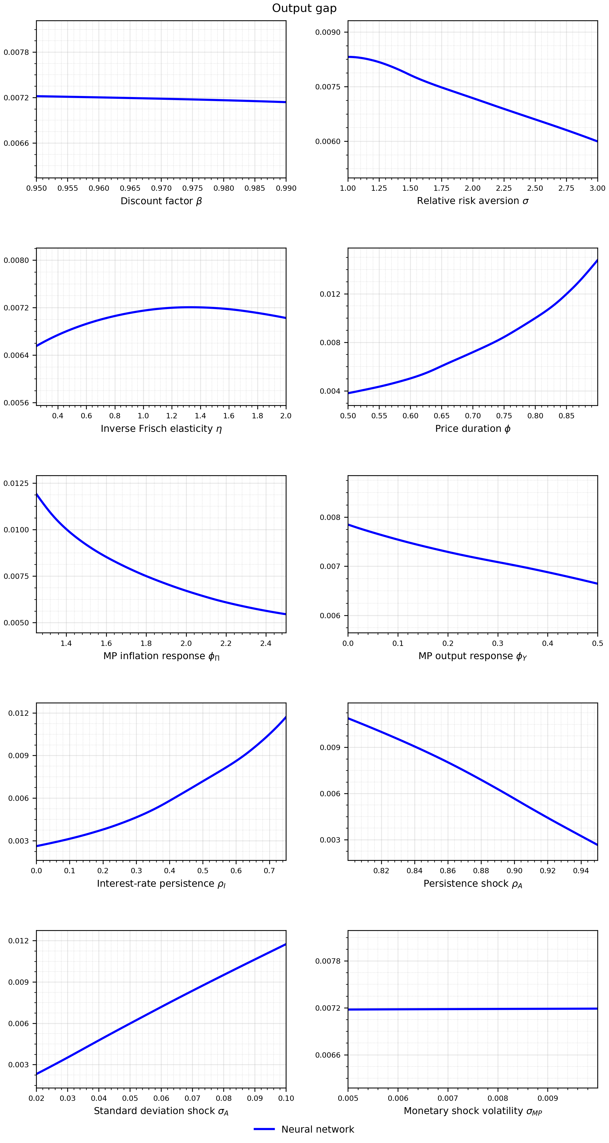
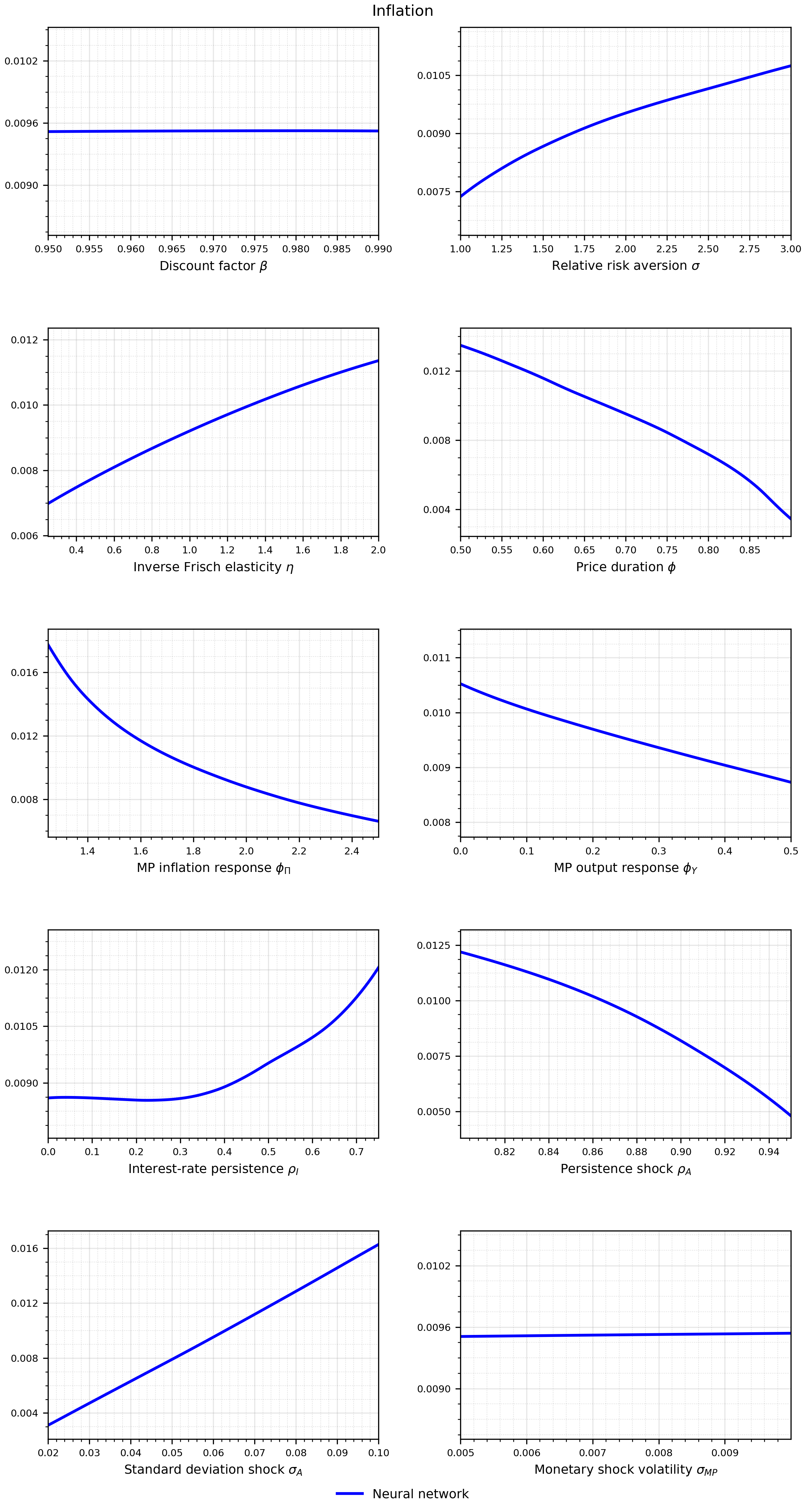
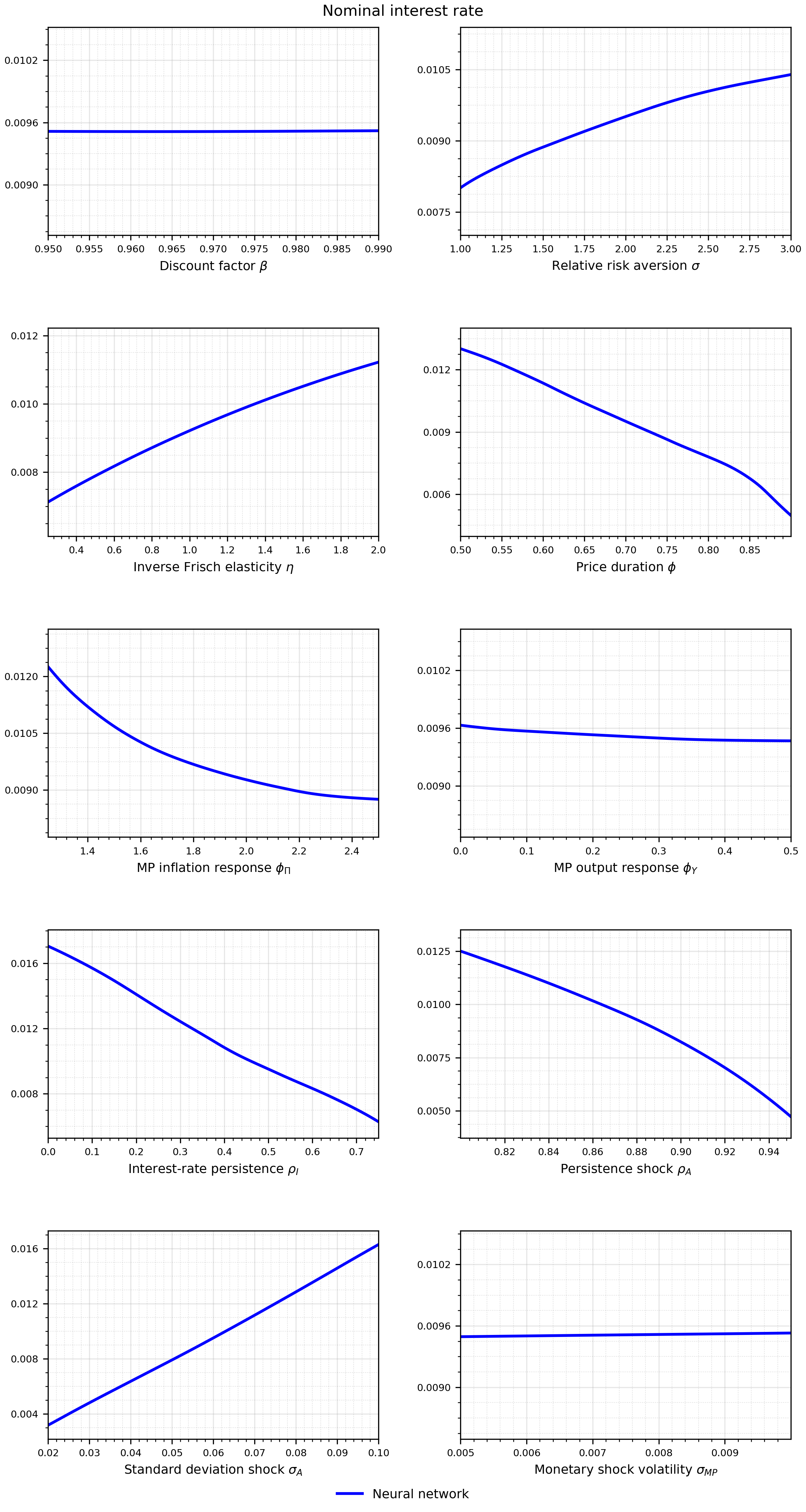
Likelihood