Extension 8: Policy network options
We now change the policy network and its training settings.
Model
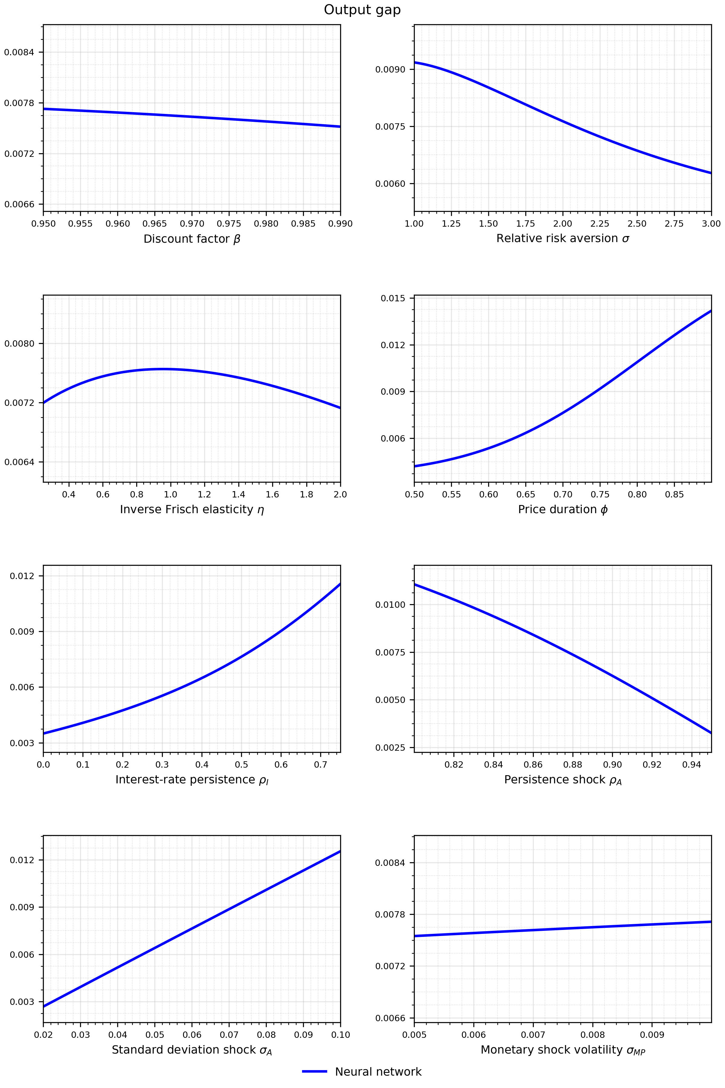
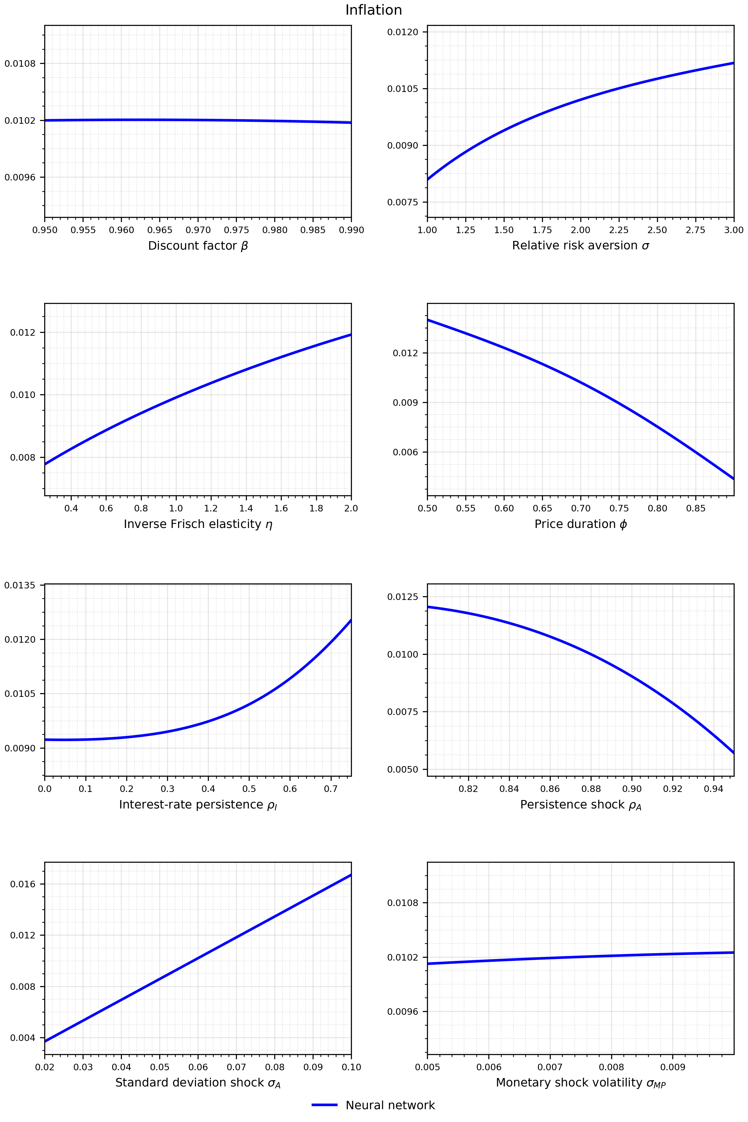
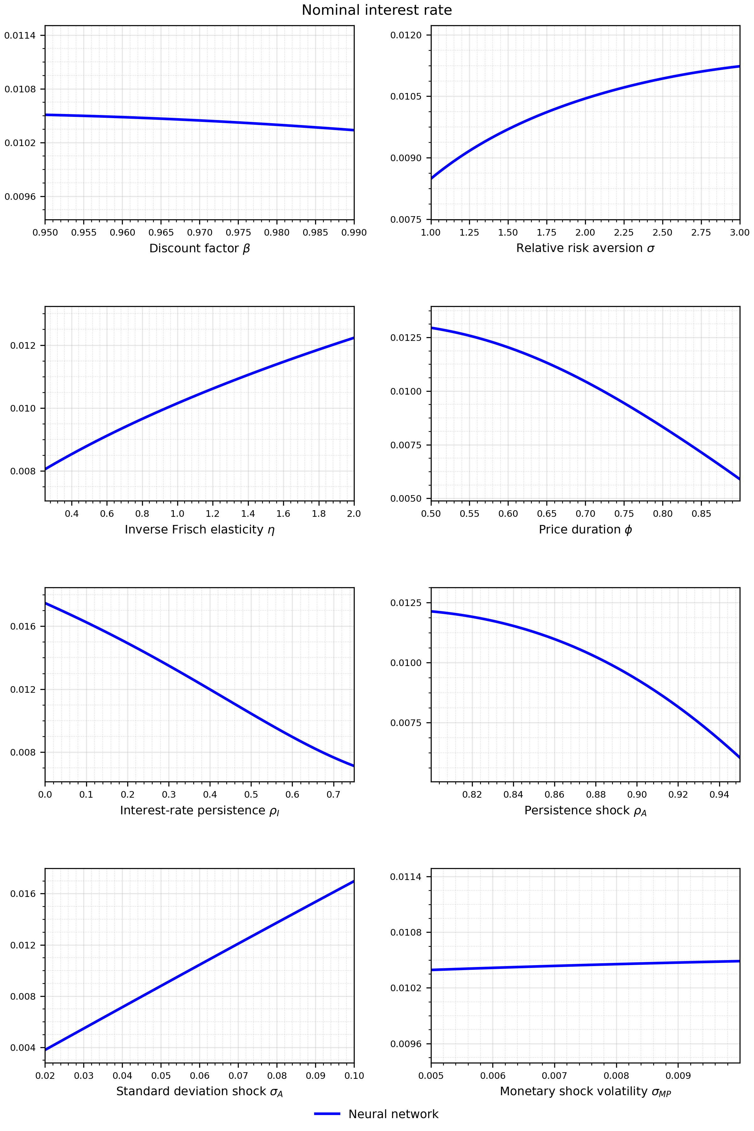
We retain the economy and transformed observation equation of Extension 7. We are now adapting various options, attributes, and hyperparameters for the training of the neural network for the extended policy functions. The suggested changes here are not necessarily improvements or optimal choices. Instead, the idea is to show the vast array of options that are available to fine-tune the learning process. After training, we need to check the accuracy of the solution again.
Neural network solution
Formulation
The focus is on the following points.
Activation function. The default choice for the activation function is CELU (Continuously Differentiable Exponential Linear Unit),
\[\text{CELU}(x)=\max(0,x)+\min\bigl(0,\alpha(\exp(x/\alpha)-1)\bigr),\]
where we set \(\alpha=1.0\) (Barron, 2017). The activation function can be easily adapted to other common alternatives such as ReLU (rectified linear unit), PReLU (parametric ReLU), sigmoid, SiLU (sigmoid linear unit), Mish (a self-regularized, non-monotonic activation function), Softplus, or Tanh (hyperbolic tangent), among others. The full list of options is in the PyTorch documentation under non-linear activations. In this extension, we change the activation function to SiLU.
Width and depth. The policy network has 64 neurons in each of 5 hidden layers in the baseline. In this extension, we increase the number of neurons to 128 and decrease the number of hidden layers to 4. One way to cross-check that the neural network is sufficiently complex to capture the dynamics is to ensure that the results do not change when increasing the width and depth.
Optimizer. Our default optimizer is AdamW (Loshchilov and Hutter, 2017), a modified version of the Adam (adaptive moment estimation) optimizer (Kingma and Ba, 2014). AdamW modifies the weight decay relative to Adam. In this extension, we change the optimizer to Adam.
Loss function criterion. The neural network minimizes a set of equations. The error in the equations can be evaluated by different criteria. All examples use the mean squared error, with a weight of 1,000 on each equation, as explained in the baseline’s training settings. Another option is the Huber loss, which is less sensitive to outliers. It would replace the squares in loss. PyTorch offers several such criteria, for example SmoothL1Loss.
Policy function transformation. The neural network provides an output at the last layer, and we can transform this outcome. In the baseline, we scale the output down by dividing it by 100. The output could also be transformed using activation functions or constrained between some bounds. In this extension, we use the hyperbolic tangent to transform the network output, which bounds it between \(-1\) and \(1\). It is important to ensure that this transformation aligns with the underlying economic model. An appropriate scaling can help to find a solution.
Input normalization. We normalize the inputs, our state variables, before feeding them into the neural network to facilitate the optimization. While we initially set the bounds of the state variables to \([-0.025,0.025]\), we widen them here to \([-1,1]\). This normalization does not clip the state. The parameters are normalized with their training ranges automatically, so they are not an option here.
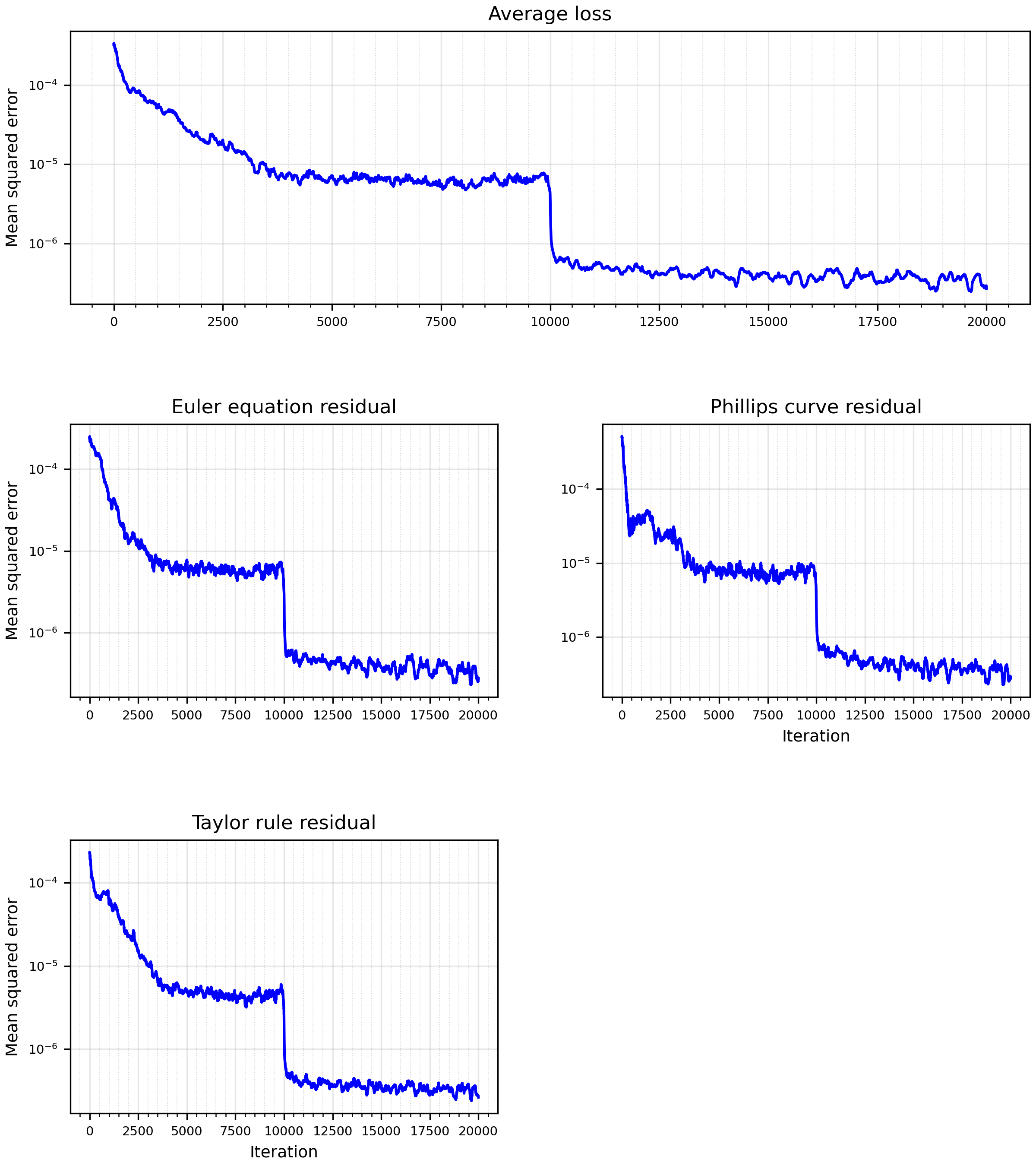
Number of iterations. The baseline trains for 10,000 iterations. The main intention behind this choice is to get the neural network reasonably trained in a limited time. We now increase the training length to 20,000 iterations.
Learning rate. We impose a schedule for the learning rate, which determines the step size during each iteration. In the baseline, we use cosine annealing, which lowers the learning rate from \(10^{-3}\) to \(10^{-10}\) along a cosine curve. In this extension, we multiply the learning rate by 0.1 every 10,000 iterations using the StepLR scheduler.
Batch size. We initially use a batch of 500 economies. In this extension, we lower it to 100.
Drawing new parameter values for the pseudo-state variables. The baseline redraws the parameter values after every iteration. Particularly for more complex models, there is a trade-off between varying the parameter values and staying in the right stochastic solution domain, as it takes time to converge to the state space when simulating forward. In this extension, we redraw the parameters every 10 iterations.
Stochastic solution domain and simulation steps. We draw the training states by simulating the model forward with our neural network solution. The baseline uses 10 simulation steps per iteration. For the purpose of this exercise, we lower them to 5.
Monte Carlo integration. We use Monte Carlo integration to approximate expectations. The baseline uses 2 draws for the next period, a single antithetic pair. Once trained, the policies are linear and the pair is exact, but during training the network is not exactly linear. We raise the number of draws to 10. As we use antithetic variates when drawing the shocks, the number of draws must be even.
Internal optimization steps. Several internal optimization steps increase the precision of the expectations. We conduct several optimization rounds with new sets of shock draws to evaluate expectations, while we fix the current state variables. The baseline runs five internal optimization steps. In this extension, we reduce them to 2.
The table summarizes the changes.
| Setting | Extension 7 | This extension |
|---|---|---|
| Activation | CELU | SiLU |
| Hidden layers | 5 of 64 units | 4 of 128 units |
| Output transformation | Divide by 100 | \(\tanh\) |
| State normalization bounds | \(\pm0.025\) | \(\pm1\) |
| Optimizer | AdamW | Adam |
| Learning rate | \(10^{-3}\), cosine to \(10^{-10}\) | \(10^{-3}\), multiplied by 0.1 every 10,000 iterations |
| Iterations | 10,000 | 20,000 |
| Batch of economies | 500 | 100 |
| Redraw parameters | Every iteration | Every 10 iterations |
| Simulate forward | 10 periods per iteration | 5 periods per iteration |
| Monte Carlo draws | 2, one antithetic pair | 10, with antithetic pairs |
| Internal updates | 5 per iteration | 2 per iteration |
| Loss | MSE, equation weights 1,000 | Unchanged |
In the code
Normalize inputs and transform outputs
state_bounds controls input scaling, and the defaults of make_network set the new layers and activation. policy evaluates the network, names its outputs, and applies tanh separately to each prediction.
examples/rank/rank_extension_08.py
def state_bounds(self):
    # New in Extension 8: wider normalization bounds.
    return torch.tensor([-1.0, -1.0, -1.0]), torch.tensor([1.0, 1.0, 1.0])

# New in Extension 8: four hidden layers of 128 SiLU units.
def make_network(self, hidden=128, layers=4, activation=torch.nn.SiLU):
    """Normalize states and parameters, then apply a fully connected network."""
    layer_list = []

    # Normalize layer
    state_low, state_high = self.state_bounds()
    # New in Extension 5: only the parameters with a range are inputs.
    keys = self.ranges.keys_estimable()
    low = torch.cat((state_low, self.ranges.low_tensor(keys)))
    high = torch.cat((state_high, self.ranges.high_tensor(keys)))
    layer_list.append(NormalizeLayer(low, high))

    # First layer
    layer_list.append(torch.nn.Linear(len(low), hidden))
    layer_list.append(activation())

    # Middle layers
    for _ in range(1, layers):
        layer_list.append(torch.nn.Linear(hidden, hidden))
        layer_list.append(activation())

    # Last layer
    layer_list.append(torch.nn.Linear(hidden, len(self.POLICY_NAMES)))

    return torch.nn.Sequential(*layer_list)
examples/rank/rank_extension_08.py
def policy(self, state=None, par=None):
    state = self.state if state is None else state
    par = self.par_draw if par is None else par

    # Vectors of states and parameters.
    states = state.cat(keys=self.STATE_NAMES)
    # New in Extension 5: pass only the parameters with a range.
    parameters = par.cat(keys=self.ranges.keys_estimable())

    # Future states have an extra leading dimension for the shock draws.
    # Repeat the parameters along it to evaluate expectations.
    if states.dim() > parameters.dim():
        parameters = parameters.expand(states.shape[0], *parameters.shape)

    # Evaluate the network on the combined inputs.
    inputs = torch.cat((states, parameters), dim=-1)
    output = self.network(inputs)

    # New in Extension 8: bound each prediction between -1 and 1 instead of dividing by 100.
    X = torch.tanh(output[..., 0:1])
    Pi = torch.tanh(output[..., 1:2])
    I = torch.tanh(output[..., 2:3])

return X, Pi, IChoose the optimizer and schedule
train_model builds the optimizer, which changes the network weights at each internal update, and the schedule, which changes the learning rate after each outer iteration. The two lines marked New in Extension 8 are all that changes in the training loop.
examples/rank/rank_extension_08.py
def train_model(self, config):
    """Train the policy network with the settings in config."""
    seed_all(config.seed)
    self.training_conf = config

    # Set the network to train mode.
    self.network.train()
    self.to(config.device)

    # Draw parameters and initial states.
    par_draw = self.draw_parameters((config.batch, 1), device=config.device)
    self.prepare(par_draw, batch=config.batch, device=config.device)

    # Starting weights for the equations.
    weights = config.weights.initial(len(self.RESIDUAL_NAMES))
    weight_state = None

    # Optimizer and scheduler.
    # New in Extension 8: Adam and a step learning-rate schedule.
    optimizer = torch.optim.Adam(self.network.parameters(), lr=config.lr)
    scheduler = torch.optim.lr_scheduler.StepLR(optimizer, step_size=10000, gamma=0.1)

    # Loss history: the total, each equation, and each equation weight.
    self.loss_dict = {"iteration": [], "total": []}
    for name in self.RESIDUAL_NAMES:
        self.loss_dict[name] = []
        self.loss_dict[f"w_{name}"] = []

    # Training loop.
    pbar = trange(config.iteration)
    running_loss = 0.0
    for i in pbar:
        # Update the network several times on the same states, with new shocks each time.
        for o in range(config.inner_steps):
            optimizer.zero_grad()
            shape = (config.mc, config.batch, 1)
            e = self.draw_shocks(shape, antithetic=True, device=config.device)
            residuals = self.residuals(e, config.detach_next)
            loss, components = self.loss(residuals, weights)
            loss.backward()
            torch.nn.utils.clip_grad_norm_(self.network.parameters(), 1.0)
            optimizer.step()

            # Record the first update, before the network adapts to these states.
            if o == 0:
                self.loss_dict["iteration"].append(i)
                self.loss_dict["total"].append(loss.item())
                for name, weight in zip(self.RESIDUAL_NAMES, weights):
                    self.loss_dict[name].append(components[name])
                    self.loss_dict[f"w_{name}"].append(weight)
                running_loss += loss.item()

        # Update adaptive weights. Fixed weights stay unchanged.
        losses = list(components.values())
        weights, weight_state = config.weights.update(
            weights, losses, i, warmup_iter=None, state=weight_state)

        # Show the running loss in the progress bar.
        if i % config.print_after == 0:
            pbar.set_postfix({
                "loss": running_loss / config.print_after,
                "lr": scheduler.get_last_lr()[0],
            })
            running_loss = 0.0

        # Update the learning rate.
        scheduler.step()

        # Draw new parameters.
        if i % config.par_draw_after == 0:
            self.par_draw = self.draw_parameters((config.batch, 1), device=config.device)
            self.ss = self.steady_state()

        # Sample new states by simulation.
        self.steps(config.batch, config.device, config.steps)

    # Set the network to evaluation mode.
    self.network.eval()
self.to("cpu")Set training counts
The notebook passes these settings to the model’s training loop.
examples/rank/rank_extension_08.py
model = NKModelExt8(PARAMETERS, RANGES, SHOCKS)
model_path = folder / "model.pt"
train_model = not load_model or not model_path.exists()

training_config = TrainingConfig(
    iteration=20000,
    inner_steps=2,
    steps=5,
    batch=100,
    mc=10,
    par_draw_after=10,
    lr=1e-3,
    device=DEVICE,
    seed=1234,
    weights=ConstantWeights([1000.0, 1000.0, 1000.0]),
    detach_next=True,
)

if train_model:
    print("Training the policy network...")
    model.train_model(training_config)
    # A new policy needs new observations, so delete the saved ones.
    (folder / "observations.pt").unlink(missing_ok=True)
    model.save(model_path)
else:
    print("Loading the saved policy network.")
model.load(model_path)Results
Solution
Likelihood