Extension 9: Filtering options
We now change the settings for the particle filter and the likelihood network.
Model
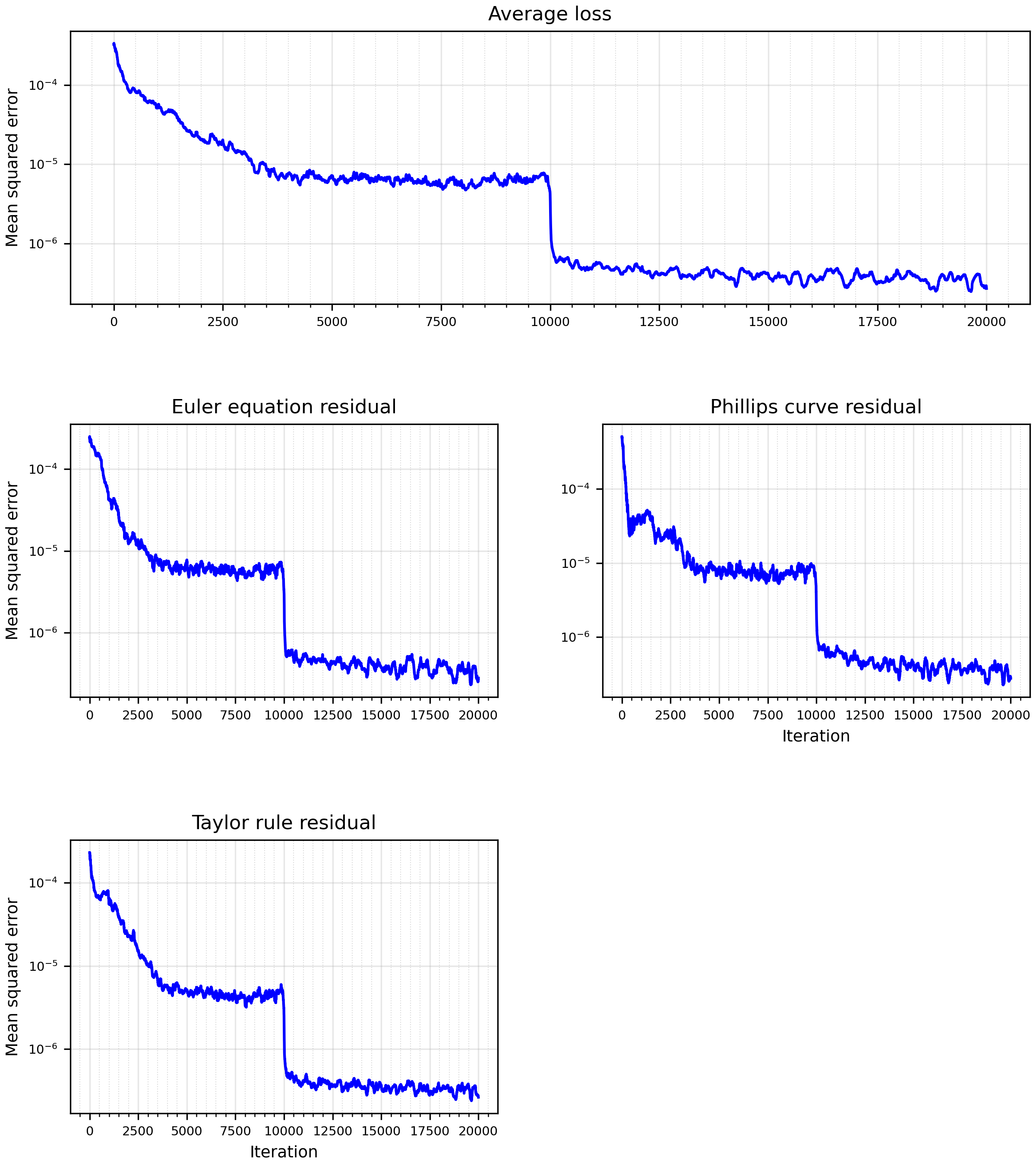
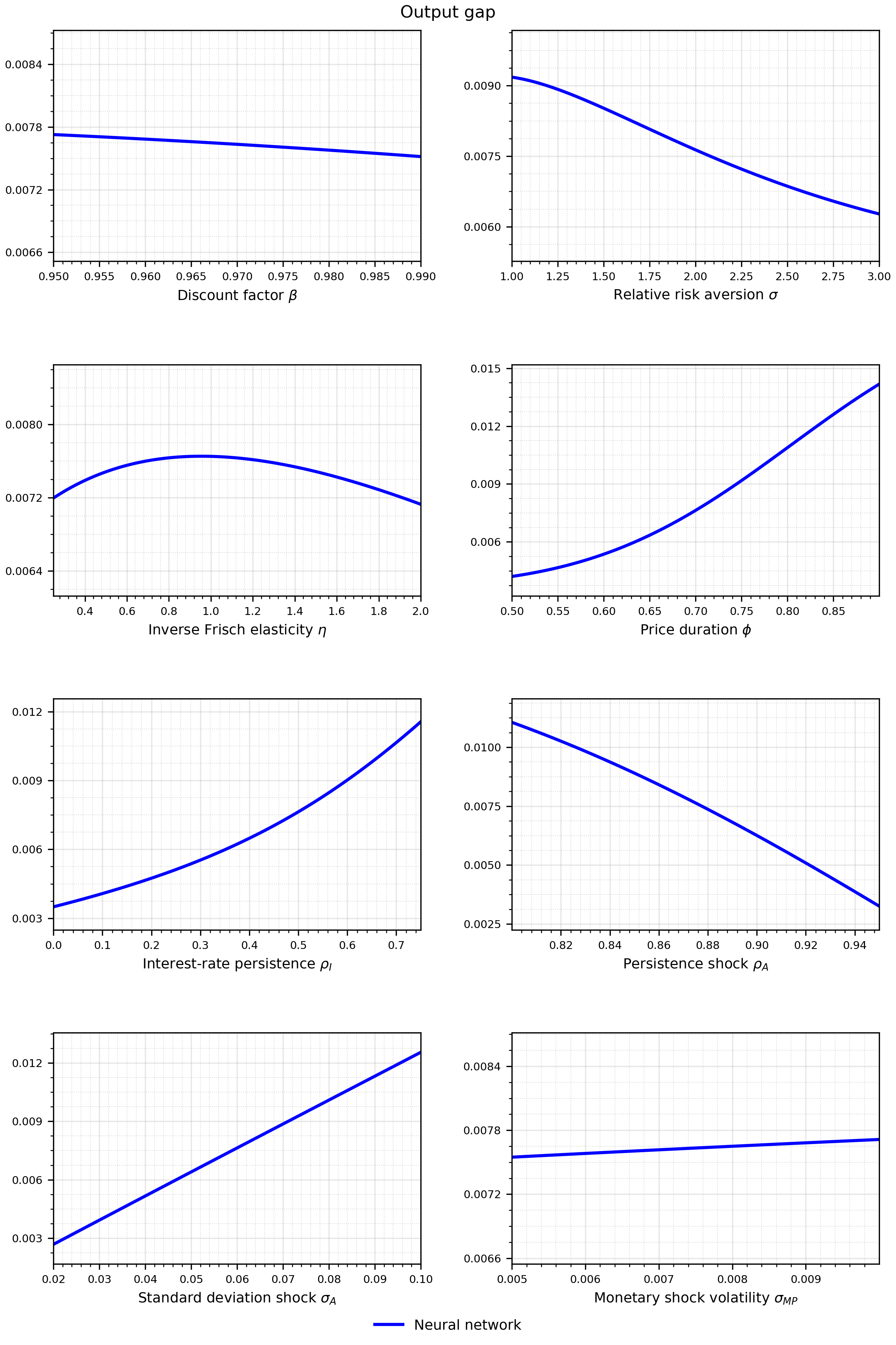
The economy and policy solution are those of Extension 8. We are now adapting various options, attributes, and hyperparameters of the setup and of the training of the neural network for the filtering step. Some options are the same as for the solution step, so we keep their explanation short. As before, the suggested changes here are not necessarily improvements or optimal. Instead, the idea is to show the vast options that are available to fine-tune the learning process.
Neural network solution
Formulation
For parameter draw \(\Theta_n\), the particle filter provides a log-likelihood target \(\widehat\ell_n\). The likelihood network \(\ell_\omega\) minimizes
\[\mathcal L_{\ell}(\omega)=\frac{1}{N_{\text{train}}}\sum_{n\in\text{train}} \left[\ell_\omega(\Theta_n)-\widehat\ell_n\right]^2.\]
The focus is on the following points for the likelihood network.
Activation function. While the activation function in the baseline is CELU, this extension uses the self-regularized, non-monotonic activation function Mish.
Width and depth. We increase the number of neurons to 256 per layer and the number of hidden layers from 3 to 5.
Optimizer. We change the optimizer from AdamW to Adam, as in the previous extension.
Batch. We increase the batch size from 100 to 200.
Epochs. We lower the number of training epochs, each a complete pass through the training data, from 5,000 to 3,000.
Number of draws. Initially, we used 5,000 draws from the parameter space and calculated the likelihood at each with the particle filter. In this extension, we increase the number of draws to 7,500.
Size of the validation sample. The drawn points are divided into a training and a validation sample, which helps to detect overfitting. While we initially used 20% of the points for validation, we increase the share to 25%.
Learning rate. As in the solution step, we change the learning-rate scheduler. We multiply the learning rate by 0.1 every 1,000 epochs using the StepLR scheduler.
In addition to the neural network setup, a few options are specific to the particle filter and the creation of the data.
Measurement error. The measurement error \(u_t\) affects the observation equation and helps to avoid degeneracy of the likelihood. In this extension, we lower its variance to \(m_E=0.05\) of each series’ variance.
Number of particles. We increase the number of particles from 100 to 250.
Length of the data. Each likelihood target initially used 100 periods of the simulated data. We increase this to 125 periods.
The table summarizes the changes.
| Setting | Extension 8 | This extension |
|---|---|---|
| Parameter draws | 5,000 | 7,500 |
| Particles per target | 100 | 250 |
| Observations per target | 100 | 125 |
| Measurement-error share \(m_E\) | 0.25 | 0.05 |
| Likelihood network | 3 hidden layers of 64 CELU units | 5 hidden layers of 256 Mish units |
| Optimizer and schedule | AdamW, cosine | Adam, multiplied by 0.1 every 1,000 epochs |
| Epochs | 5,000 | 3,000 |
| Batch | 100 | 200 |
| Validation share | 20% | 25% |
The policy loss is unchanged from Extension 1.
In the code
Generate likelihood targets
Each parameter vector requires one particle-filter evaluation. Using more particles reduces simulation noise but takes more time. sim=125 uses the first 125 of the 1,000 simulated observations, and burn=100 runs the particles forward 100 periods before filtering starts.
examples/rank/rank_extension_09.py
surrogate_path = folder / "surrogate.pt"
train_pf_network = not load_pf_network or not load_pf_dataset or make_data or not surrogate_path.exists()
make_pf_dataset = train_pf_network and (not load_pf_dataset or make_data or not pf_dataset_path.exists())

if make_pf_dataset:
    print("Generating likelihood targets...")
    pf.generate_likelihood_dataset(
        N=7500, P=250, sim=125, burn=100, sobol=True, device=DEVICE, seed=12345,
    )
    pf_dataset_path.parent.mkdir(parents=True, exist_ok=True)
    torch.save(pf.dataset, pf_dataset_path)
elif train_pf_network:
    print("Loading the saved likelihood targets.")
pf.dataset = torch.load(pf_dataset_path, weights_only=True)Specify and train the likelihood network
train fits the likelihood network. Validation draws are excluded from weight updates, although the output-scaling bounds use the full target dataset. Set only load_pf_network = False to retrain the network using saved likelihood targets.
Choose the number of epochs with the dataset and batch sizes in mind. If validation loss keeps rising while training loss falls, the likelihood network may be overfitting. Training keeps the weights from the final epoch and does not select the best validation epoch.
examples/rank/rank_extension_09.py
if train_pf_network:
    (folder / "likelihood_sigma.pt").unlink(missing_ok=True)
    (folder / "likelihood_all.pt").unlink(missing_ok=True)
    print("Training the likelihood network...")
    pf.make_surrogate_network(hidden=256, layers=5, activation="Mish", seed=1234)
    pf.train(
        batch=200, epochs=3000, lr=1e-3,
        validation_share=0.25, print_after=100, device=DEVICE, seed=1234,
        optimizer_name="Adam", scheduler_name="step", step_size=1000, gamma=0.1,
    )
    pf.dataset = None  # Targets are stored separately in pf_dataset_path.
    pf.save(folder, name="surrogate")
else:
    print("Loading the saved likelihood network.")
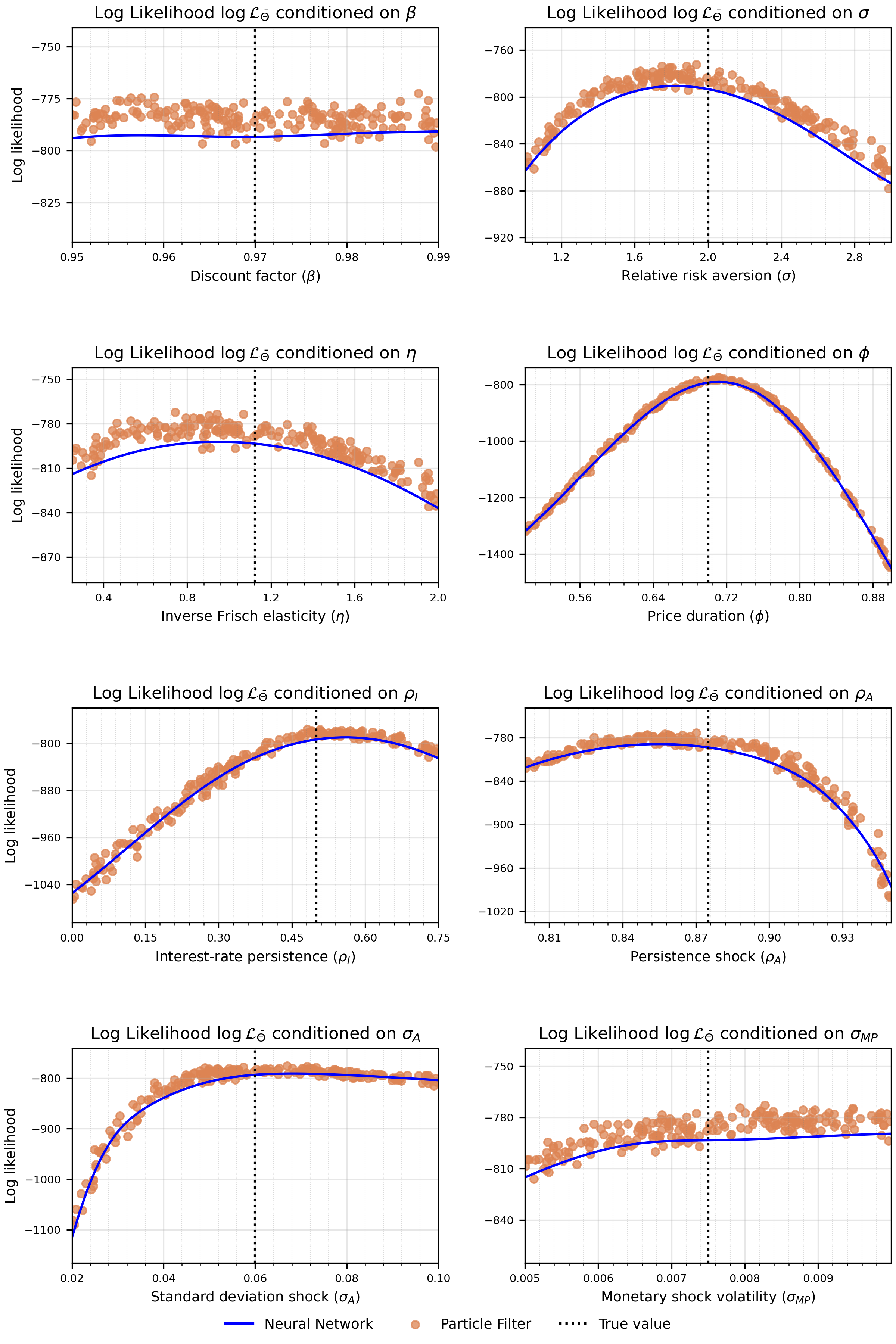
pf.load(surrogate_path)The notebook plots the training and validation MSE and compares the likelihood network with particle-filter evaluations at random parameter values, using the new 250 particles and 125 observations. Both use the same learned policy, so this comparison checks the likelihood approximation, not the accuracy of the policy solution.
Results
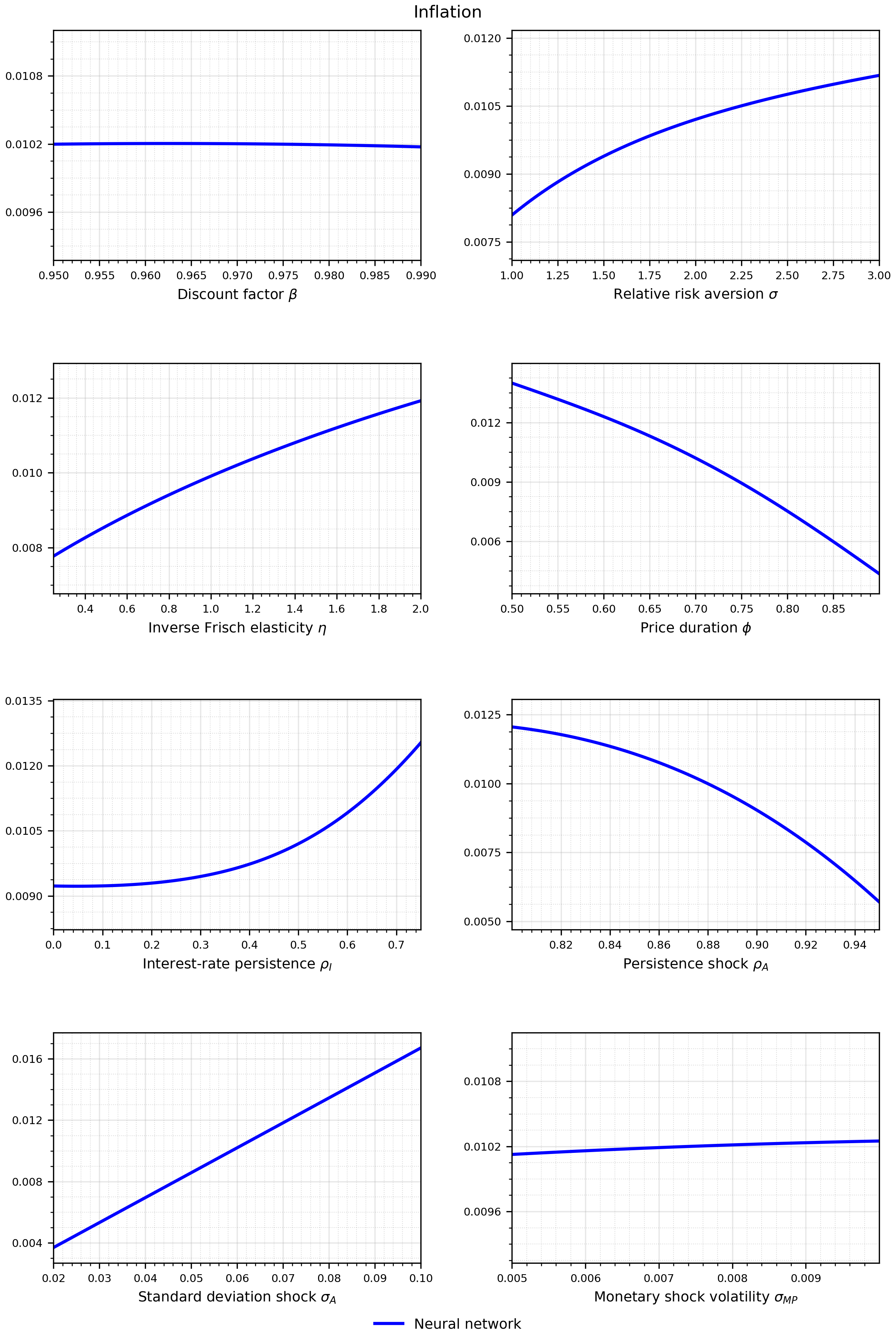
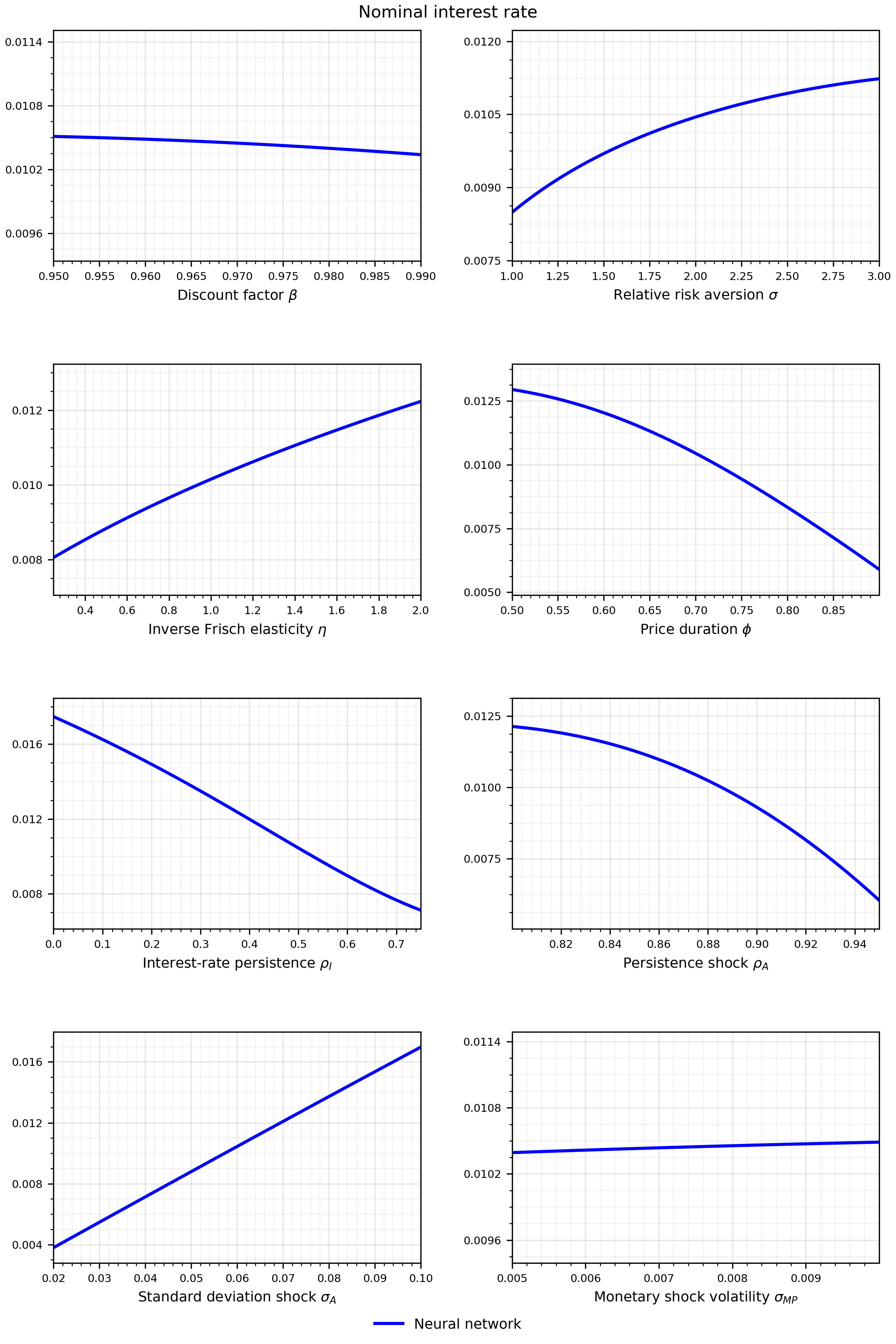
Solution
Likelihood
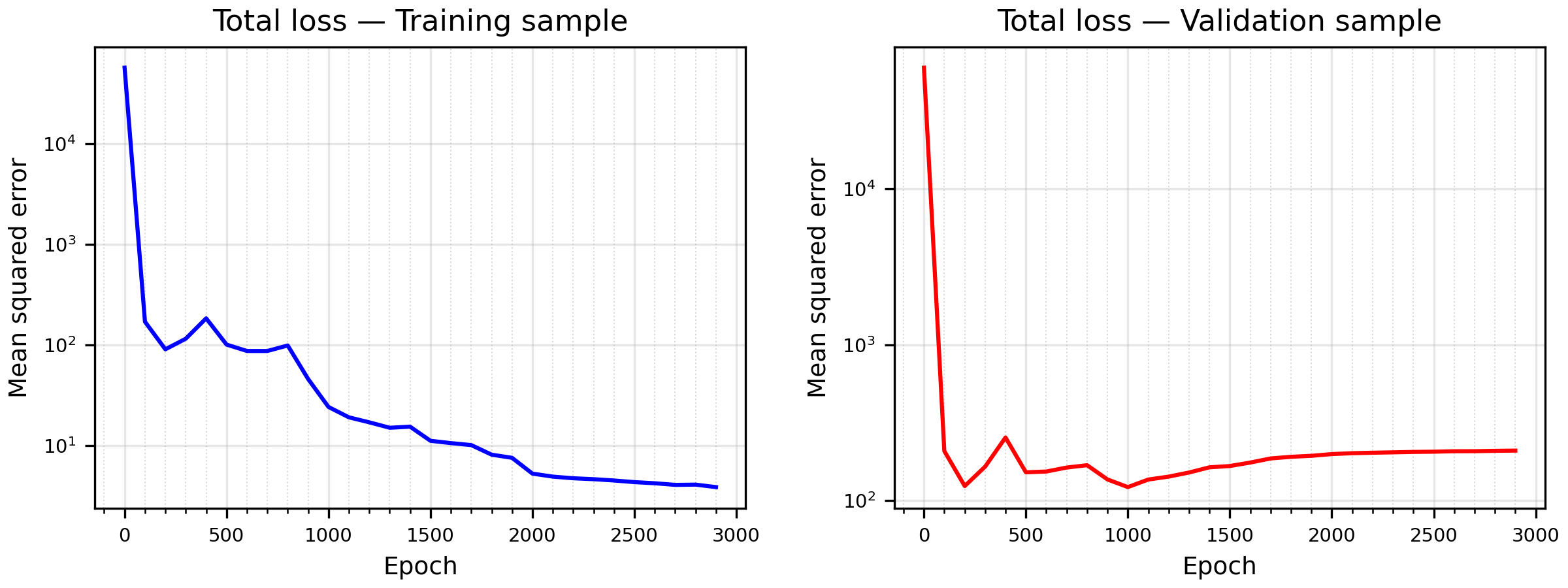
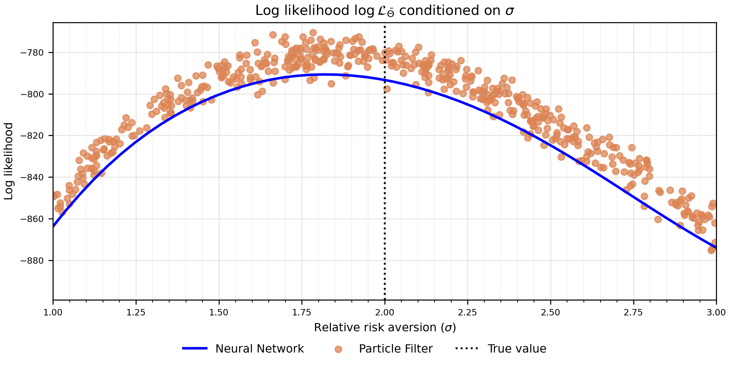
The validation loss points to overfitting. The training loss keeps falling, while the validation loss reaches its minimum after about 1,000 epochs and then rises. The larger network fits the noise in its training targets, so the curves below sit several units below the particle-filter evaluations.