Extension 2: Parameters
We add the parameter \(\rho_I\) to the Taylor rule. For now it multiplies zero, and the next extension puts the lagged interest rate in its place.
Model
\[ \begin{aligned} \hat X_t &= E_t\hat X_{t+1}-\sigma^{-1}\left(\hat I_t-E_t\hat\Pi_{t+1}-\hat R_t^*\right),\\ \hat\Pi_t &= \kappa\hat X_t+\beta E_t\hat\Pi_{t+1},\\ \hat I_t &= \rho_I\cdot 0+(1-\rho_I)\left(\phi_\Pi\hat\Pi_t+\phi_Y\hat X_t\right),\\ \hat R_t^* &= \rho_A\hat R_{t-1}^*+\sigma(\rho_A-1)\omega\sigma_A\epsilon_t^A. \end{aligned} \]
The lower and upper bounds for \(\rho_I\) are \(-0.1\) and \(0.1\).
Neural network solution
Formulation
We add \(\rho_I\) to the estimated parameter set, before the parameters of the shock process,
\[ \tilde\Theta=\{\beta,\sigma,\eta,\phi,\phi_\Pi,\phi_Y,\rho_I,\rho_A,\sigma_A\}. \]
The state, shocks, and policy outputs are unchanged. The analytical solution used in the earlier examples applies to the original Taylor rule, so we omit that comparison from this extension onward.
In the code
Add a parameter input
The new parameter is named rho_i. We insert it before rho_a and sigma_a, the two shock parameters. Its reference value is zero and its training range is \([-0.1, 0.1]\). The complete parameter lists are shown below. The other values and ranges are unchanged.
examples/rank/rank_extension_02.py
# Reference values. They also generate the data later on.
PARAMETERS = {
    "beta": 0.97,
    "sigma": 2.0,
    "eta": 1.125,
    "phi": 0.7,
    "phipi": 1.875,
    "phiy": 0.25,
    "rho_i": 0.0,  # New in Extension 2: Taylor-rule persistence.
    "rho_a": 0.875,
    "sigma_a": 0.06,
}

# Training ranges. Every parameter with a range is a network input.
RANGES = {
    "beta": torch.distributions.Uniform(0.95, 0.99),
    "sigma": torch.distributions.Uniform(1.0, 3.0),
    "eta": torch.distributions.Uniform(0.25, 2.0),
    "phi": torch.distributions.Uniform(0.5, 0.9),
    "phipi": torch.distributions.Uniform(1.25, 2.5),
    "phiy": torch.distributions.Uniform(0.0, 0.5),
    "rho_i": torch.distributions.Uniform(-0.1, 0.1),
    "rho_a": torch.distributions.Uniform(0.8, 0.95),
    "sigma_a": torch.distributions.Uniform(0.02, 0.1),
}Every parameter with a range is a network input, so adding rho_i also adds one input.
Adjust the Taylor rule
The complete residual calculation is below. It evaluates current policies, computes next-period expectations, and checks all three equations. The new factor 1 - rho_i appears in the Taylor-rule residual. The Euler equation and Phillips curve keep their previous form.
examples/rank/rank_extension_02.py
def residuals(self, e, detach_next=True):
    par = self.par_draw

    # Evaluate today's policies.
    X, Pi, I = self.policy()

    # Next period's state for each shock draw.
    state_next = self.next_state(e)

    # Evaluate next period's policies at that state.
    with torch.set_grad_enabled(not detach_next):
        X_next, Pi_next, _ = self.policy(state_next)

    # Average over the draws to approximate the conditional expectations.
    EX_next = X_next.mean(dim=0)
    EPi_next = Pi_next.mean(dim=0)

    # F_1: Euler equation.
    euler = X - (EX_next - (I - EPi_next - self.state.zeta) / par.sigma)
    # F_2: Phillips curve.
    phillips = Pi - (self.ss.kappa * X + par.beta * EPi_next)
    # F_3: Taylor rule. New in Extension 2: scale the policy response by (1 - rho_I).
    taylor = I - (1 - par.rho_i) * (par.phipi * Pi + par.phiy * X)
return [euler, phillips, taylor]At rho_i = 0, this rule reduces to Extension 1’s rule. No new policy output or state is needed.
Results
Solution
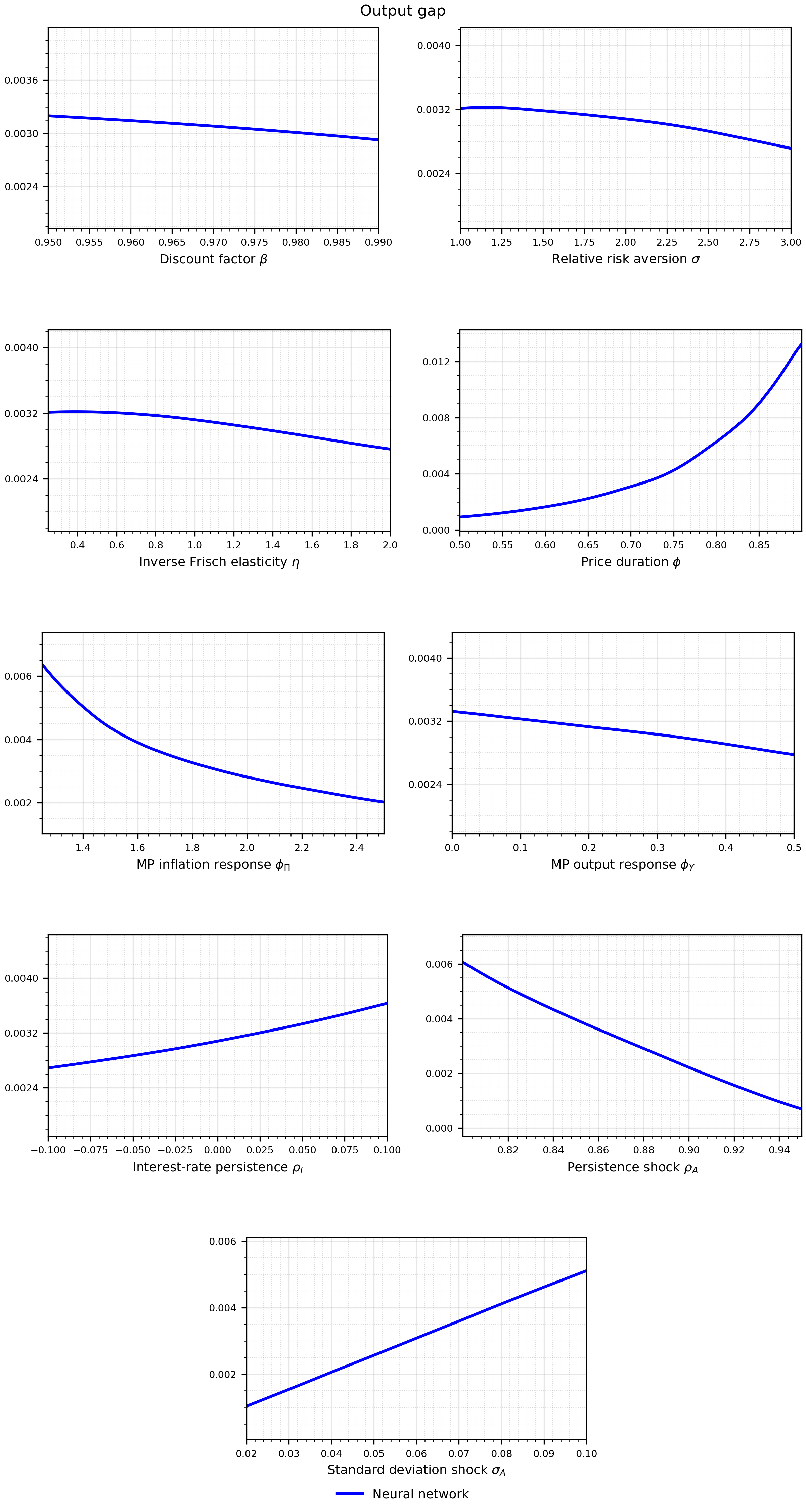
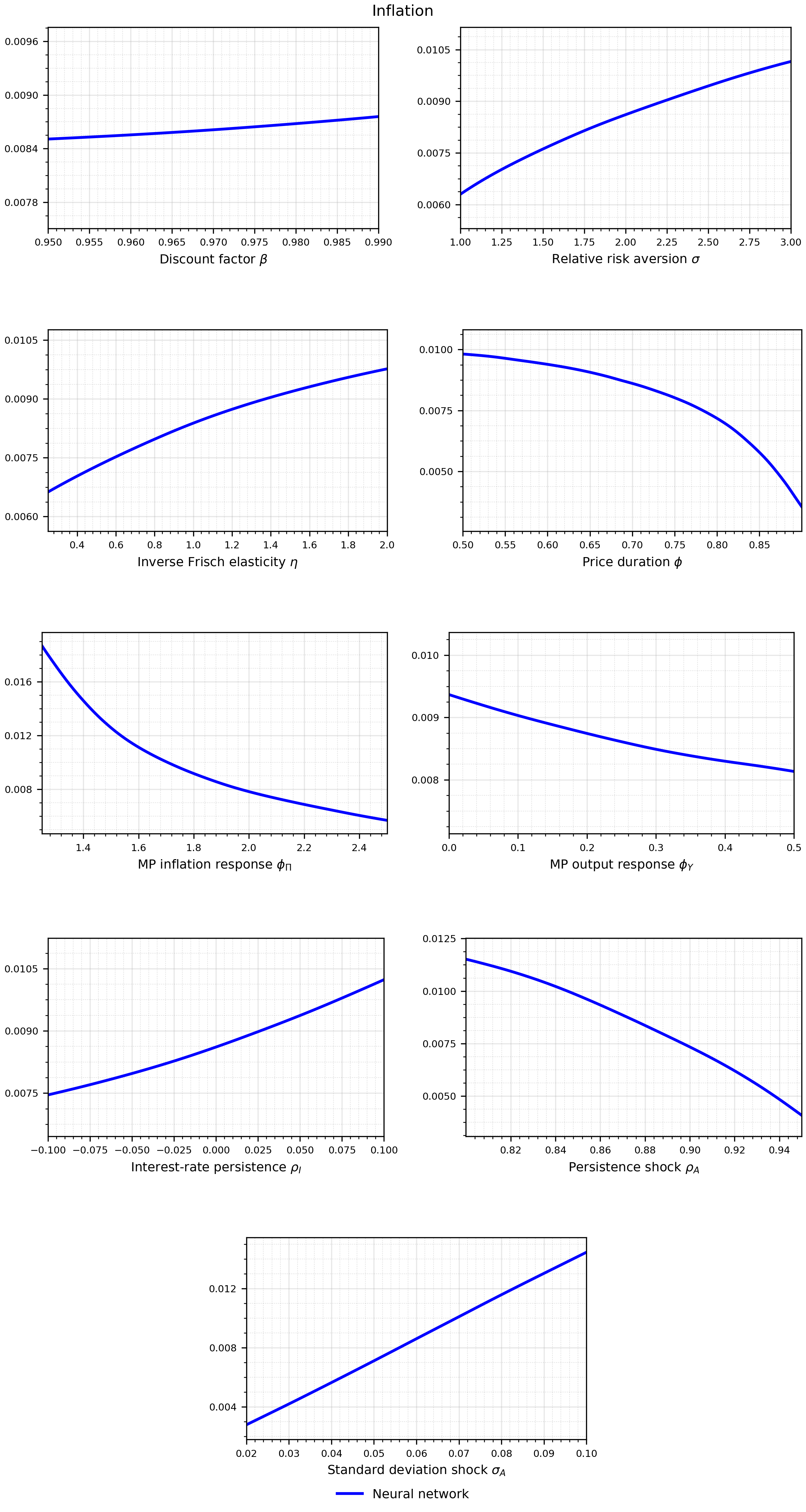
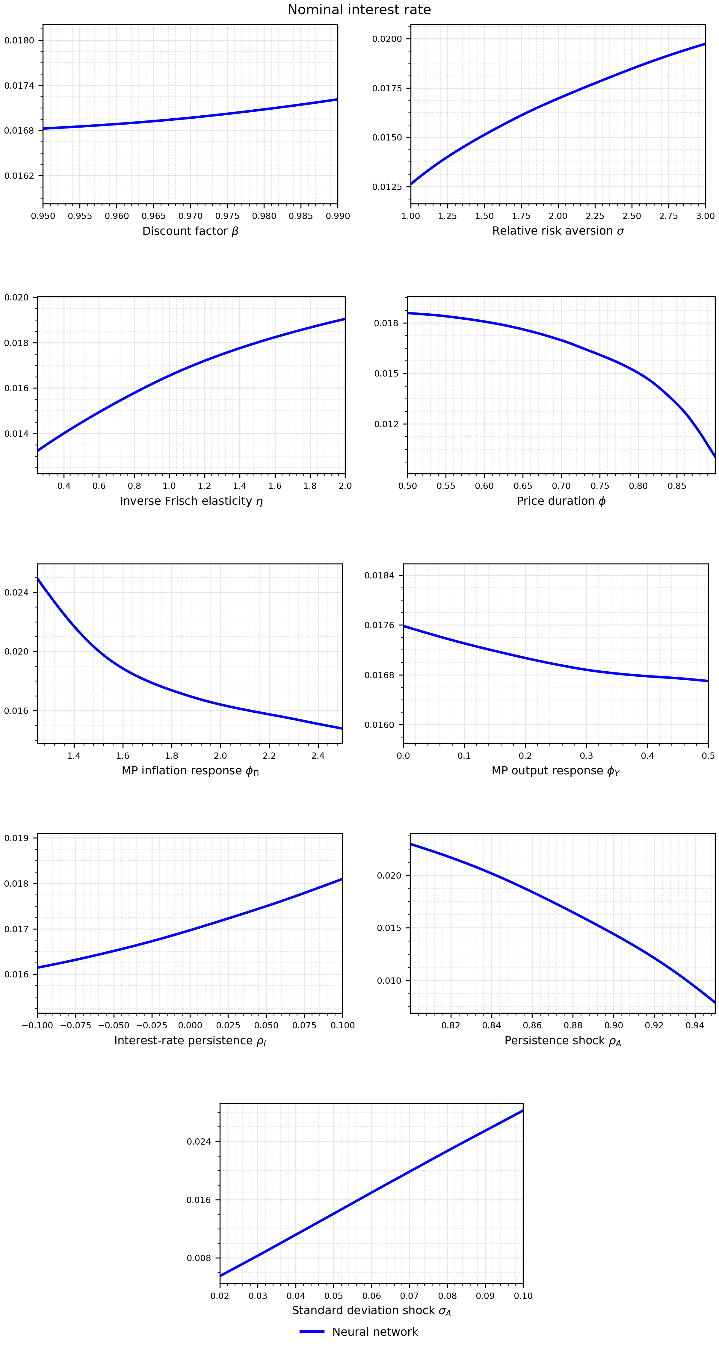
Likelihood