Krusell–Smith: one asset
The next model in the learning path is a heterogeneous agent model with aggregate risk. Specifically, it is the stochastic growth model with partially uninsurable income risk based on Krusell and Smith (1998). However, we abstract from cyclical income risk.
We solve the model using neural networks. We use 100 agents (\(L=100\)) to approximate the distribution. The model itself is solved in two steps. We first solve the deterministic steady state. Afterward, we solve the full equilibrium of the model. Finally, we compare the results to the ones obtained with the sequence-space Jacobian (SSJ) approach of Auclert et al. (2021). For ease of comparison, we follow their setup of the model.
The script coordinates separate model, analysis, and plotting files, as in the paper’s replication package. Its saved networks are the trained networks from that package, so the script reproduces the solution without retraining. Run it from the environment described in Setting up Python.
Model
The economy consists of a continuum of households. The households choose consumption \(C_t^i\) to maximize their utility
\[E_0\sum_{t=0}^\infty\beta^t\frac{(C_t^i)^{1-\sigma}}{1-\sigma},\]
with \(\sigma=1\), so that utility is logarithmic. The budget constraint can be written as
\[C_t^i+K_t^i=(1+r_t)K_{t-1}^i+w_t\bar H\exp(s_t^i),\]
where \(K_t^i\) is the household-specific capital, \(r_t\) is the rental rate of capital, and \(w_t\) is the wage. Each household has an endowment of labor \(\bar H\). Its individual labor productivity \(s_t^i\) is stochastic and follows an AR(1) process, \(s_{t+1}^i=\rho_s s_t^i+\sigma_s\epsilon_{t+1}^{s,i}\). The agents cannot hold capital below some limit, \(K_t^i\geq\underline K\). The first-order condition can be written as
\[1=\beta\mathbb E_t\left[\left(\frac{C_{t+1}^i}{C_t^i}\right)^{-\sigma}(1+r_{t+1})\right]+\mu_t^i,\]
where \(\mu_t^i\) is the normalized Lagrange multiplier on the borrowing constraint for individual capital holdings.
The representative firm produces output \(Y_t\) using total labor \(N_t\) and total capital \(K_{t-1}\),
\[Y_t=A_tK_{t-1}^\alpha N_t^{1-\alpha},\]
where total factor productivity follows the AR(1) process \(A_{t+1}=(1-\rho_A)A+\rho_AA_t+\sigma_A\epsilon_{t+1}^A\) around its steady-state level \(A\). The first-order conditions are
\[r_t=\alpha\frac{Y_t}{K_{t-1}}-\delta,\qquad w_t=(1-\alpha)\frac{Y_t}{N_t}.\]
Market clearing for the labor market, capital market, and goods market requires
\[N_t=\int\exp(s_t^i)\bar H\,di,\qquad K_t=\int K_t^i\,di,\qquad Y_t=\int C_t^i\,di+K_t-(1-\delta)K_{t-1}.\]
Calibration
The household and technology parameters come from the SSJ steady-state solve, and the code uses them at full precision. The SSJ calibration sets the unconditional standard deviation of log productivity to 0.5, which gives the innovation standard deviation \(\sigma_s=0.5\sqrt{1-\rho_s^2}\). We set the productivity level \(A\) so that output equals 1 in the deterministic steady state. This requires us to solve the deterministic steady state of the model, which the first stage does.
| Parameter | Value | Parameter | Value |
|---|---|---|---|
| Discount factor \(\beta\) | 0.981953 | Productivity persistence \(\rho_s\) | 0.966 |
| Risk aversion \(\sigma\) | 1 | Productivity innovation SD \(\sigma_s\) | 0.129271 |
| Capital share \(\alpha\) | 0.11 | TFP persistence \(\rho_A\) | 0.9 |
| Depreciation rate \(\delta\) | 0.025 | TFP innovation SD \(\sigma_A\) | 0.01 |
| Labor endowment \(\bar H\) | 1 | Borrowing limit \(\underline K\) | 0 |
Two numerical devices keep the simulated panel well behaved. Productivity levels \(e^{s}\) are floored at 0.25 and renormalized so that their panel mean is one, and capital has an upper bound \(\overline K=40\), which is checked not to bind after training.
Neural network solution
Formulation
The state variables and shocks of the stochastic growth model with partially uninsurable labor income are
\[\mathbb S_t=\left\{\{K_{t-1}^i\}_{i=1}^L,\{s_t^i\}_{i=1}^L,A_t\right\},\qquad \nu_t=\left\{\{\epsilon_t^{s,i}\}_{i=1}^L,\epsilon_t^A\right\}.\]
All parameters are calibrated in this example,
\[\bar\Theta=\{\beta,\sigma,\alpha,\delta,\rho_s,\sigma_s,\rho_A,\sigma_A,\underline K\},\qquad \tilde\Theta=\{\},\]
so no parameter varies during training. The calibrated values still enter the networks as constant inputs. We represent the distribution with 100 households sorted by capital, and a separate panel of \(L=100\) households evaluates the individual optimality conditions. The aggregate state also contains aggregate capital \(K_{t-1}\) and productivity \(A_t\).
The solution has two stages.
- Deterministic steady state (DSS). Idiosyncratic risk remains active while aggregate risk is absent. We use this stage to calibrate the productivity level of the model to match an output level of 1. A steady-state network returns the productivity level, \(A=\psi_{NN}^{SS}(\tilde\Theta\mid\bar\Theta)\), and a household network returns consumption, \[\left\{C_t^i=\psi_{NN}^{I,DSS}\left(\mathbb S_t^i,\mathbb S,\tilde\Theta\mid\bar\Theta\right)\right\}_{i=1}^L, \qquad\mathbb S_t^i=\{K_{t-1}^i,s_t^i\}.\] We let the aggregate state still enter the network. While this is unnecessary for solving the DSS, it allows us to use this trained network as the starting point when we solve the full equilibrium with aggregate risk.
- Full equilibrium. Initialize the household network with the DSS weights and train it with aggregate risk, \(C_t^i=\psi_{NN}^I(\mathbb S_t^i,\mathbb S_t,\tilde\Theta\mid\bar\Theta)\), while the steady-state network stays fixed.
Each network normalizes its input groups, projects them to 128 values, and adds these projections, then applies four hidden layers of 128 CELU units and a linear output layer. Consumption is the representative-agent steady-state level times \(0.2+0.8e^{o}\) of the network output \(o\), and the productivity level is the representative-agent level times a sigmoid in \([0.8,1.2]\). Capital then follows from the budget constraint,
\[K_t^i=(1+r_t)K_{t-1}^i+w_t\bar H\exp(s_t^i)-C_t^i.\]
Residuals and loss
The Fischer–Burmeister function \(\Psi^{FB}(a,b)=a+b-\sqrt{a^2+b^2}\) writes the Kuhn–Tucker conditions of the borrowing constraint. Let \(\bar\lambda_t^i=\beta\mathbb E_t[(C_t^i/C_{t+1}^i)(1+r_{t+1})]\), which the code computes as the mean over \(M\) shock draws. With the numerical upper bound \(\overline K\), the household residual is
\[F^{1,i}_t=\begin{cases} \Psi^{FB}(K_t^i-\underline K,1/\bar\lambda_t^i-1), & K_t^i<0.8\overline K,\\ \Psi^{FB}(\overline K-K_t^i,1-1/\bar\lambda_t^i), & K_t^i\geq0.8\overline K. \end{cases}\]
The second branch switches to the upper-bound complementarity condition. The upper bound provides stability to the algorithm, as it avoids an overaccumulation of assets during the training.
In the DSS stage, \(F^2=Y_t-1\) is the output normalization and \(F^3\) compares aggregate capital from the resource constraint, \(K_t=Y_t-C_t+(1-\delta)K_{t-1}\), with the mean of the household choices. \(F^3\) is tracked but has weight zero in that stage. In the full model, \(F^2\) and \(F^3\) are this capital consistency today and next period, one for each of the \(M\) shock draws. These are overidentifying restrictions. For a batch of \(N_{batch}\) economies, the loss is
\[ \mathcal L=\frac1{N_{batch}}\sum_{b=1}^{N_{batch}}\left[ \alpha_1\frac1L\sum_{i=1}^L(F^{1,i,b})^2+\alpha_2(F^{2,b})^2 +\alpha_3\frac1M\sum_{m=1}^M(F^{3,b,m})^2\right], \]
with weights \((1,1,0)\) in the DSS stage and \((1,1,1)\) in the full model.
Training
Each iteration takes 20 internal updates on a batch of \(N_{batch}=100\) economies. Each update draws \(M=50\) next-period shocks as antithetic pairs to approximate the expectations. The shocks that simulate the panel forward are not paired. After the updates, the panel advances one period during the first 1,000 iterations of a stage and 5 periods afterwards. In the full model, the aggregate shocks are amplified by 1.25 during these simulation steps, so the panel covers a wider range of aggregate states. An economy whose simulated capital leaves its bounds by more than half their distance, or whose aggregate capital is more than a factor 5 away from its steady-state level, is replaced by the panel of a healthy economy.
The DSS stage runs 10,000 iterations and the full model 20,000, both with AdamW, weight decay 0.01, and gradient-norm clipping at 1. The learning rate warms up from \(10^{-5}\) to \(10^{-4}\) over the first 10% of the iterations, then follows cosine annealing to \(10^{-8}\). The DSS stage uses the optimizer’s default \(\epsilon=10^{-8}\) and the full model \(10^{-10}\). Idiosyncratic shock standard deviations rise from 10% to 100% of their target over the first 1,000 iterations of the DSS stage. In the full model, the productivity shock starts at 10% and rises to full size between iterations 100 and 1,000.
In the code
Set the parameters and shocks
The household and technology parameters are read from the SSJ reference. ranges is empty, because no parameter varies during training.
examples/ksone/ksone.py
parameters = {
    # Household and technology, from the SSJ steady-state solve.
    "beta": ref_ss["beta"],
    "delta": ref_ss["delta"],
    "alpha": ref_ss["alpha"],
    "rho_s": ref_ss["rho_e"],
    "sigma_s": ref_ss["sd_e"] * math.sqrt(1 - ref_ss["rho_e"] ** 2),
    # Aggregate productivity shock.
    "rho_A": 0.9,
    "sigma_A": 0.01,
    # Bounds on capital.
    "k_bar": 0.0,
    "k_down": 40.0,
}

ranges = {}  # No parameter varies during training.

shocks_ind = {"s": torch.distributions.Normal(0.0, 1.0)}

shocks_agg = {"A_scale": torch.distributions.Normal(0.0, 1.0)}The code names map to the symbols above as follows.
| Code | Symbol | Meaning |
|---|---|---|
k |
\(K_t^i\) | capital |
s |
\(s_t^i\) | log productivity |
k_bar, k_down |
\(\underline K\), \(\overline K\) | bounds on capital |
A_scale |
\(A_t-A_{RA}\) | productivity, as a deviation from the representative-agent level |
Kl |
\(K_{t-1}\) | aggregate capital at the start of the period |
A_dss |
\(A\) | steady-state productivity, learned by the DSS network |
ss |
representative-agent steady state with \(Y=1\), which scales the network outputs | |
r, w, N |
\(r_t\), \(w_t\), \(N_t\) | factor prices and effective labor |
lambda_comp |
\(\bar\lambda_t^i\) | expected Euler term |
res_fb |
\(F^1\) | household Euler residual with the borrowing limit |
res_y, res_k |
\(F^2\), \(F^3\) | output normalization (DSS) and capital consistency |
res_k_next |
\(F^3\) | capital consistency next period (full model) |
_ind, _dist suffixes |
the \(L\)-household panel and the distribution panel |
Evaluate and transform policies
hh_policy evaluates the household network through _hh_consumption, which sorts the distribution by capital, assembles the input groups, and transforms the output into consumption relative to its steady-state level. dss_policy returns the productivity level relative to the representative-agent level. The output bounds help keep trial policies economically meaningful.
examples/ksone/ksone_model.py
def _hh_consumption(self, network, state_ind, state_dist, state_agg, par, mc=None):
    """Household consumption relative to steady-state consumption, above 0.2."""
    hh_output = network(**self._state_inputs(state_dist, state_agg, mc=mc, state_ind=state_ind),
                        par=self._prepare_par_input(par=par, mc=mc))
    return 0.2 + torch.exp(hh_output[..., 0:1]) / (1.0 / (1 - 0.2))

def hh_policy(self, state_ind, state_dist, state_agg, par, mc=None):
    return self._hh_consumption(self.hh_network, state_ind, state_dist, state_agg, par, mc=mc)

def dss_policy(self, par, mc=None):
    """DSS productivity level relative to the steady-state level, in [0.8, 1.2]."""
    dss_output = self.dss_network(par=self._prepare_par_input(par=par, mc=mc))
return 0.8 + torch.sigmoid(dss_output[..., 0:1]) * (1.2 - 0.8)Form the equilibrium errors
The method below evaluates current consumption for both panels, computes factor prices and each household’s capital from the budget constraint, and advances the states with the shock draws in e. It then evaluates future consumption, averages over the draws, and forms the three residuals. detach_next=True holds future-policy predictions fixed when differentiating today’s equation errors.
examples/ksone/ksone_model.py
def residuals(self, e, mc, detach_next=True, scale_ind=1, scale_agg=1):
    par, ss = self.par_draw, self.ss
    state_ind, state_dist, state_agg = self.state_ind, self.state_dist, self.state_agg

    c_ind = self.hh_policy(state_ind, state_dist, state_agg, par) * ss.C
    c_dist = self.hh_policy(state_dist, state_dist, state_agg, par) * ss.C
    A_dss = self.dss_policy(par) * ss.A
    A = state_agg.A_scale + ss.A

    C = torch.mean(c_dist, dim=-2, keepdim=True)
    Kl = state_agg.Kl
    N = ss.N * torch.mean(torch.exp(state_dist.s), dim=-2, keepdim=True)
    Y, r, w = self.factor_prices(A, Kl, N, par)

    # Budget constraint
    k_ind = (1 + r) * state_ind.k + w * torch.exp(state_ind.s) * ss.N - c_ind
    k_dist = (1 + r) * state_dist.k + w * torch.exp(state_dist.s) * ss.N - c_dist

    K = Y - C + (1 - par.delta) * Kl

    # Next period
    shape_ind = e["shocks_ind"].s.shape
    shape_dist = e["shocks_dist"].s.shape
    shape_agg = e["shocks_agg"].A_scale.shape

    s_ind_next = self._ar1_next(state_ind.s, e["shocks_ind"].s, par, scale_ind)
    s_dist_next = self._ar1_next(state_dist.s, e["shocks_dist"].s, par, scale_ind)
    A_next = (1 - par.rho_A) * A_dss + par.rho_A * (state_agg.A_scale + ss.A) + e["shocks_agg"].A_scale * par.sigma_A * scale_agg

    state_ind_next = State({"k": k_ind.expand(shape_ind), "s": s_ind_next})
    state_dist_next = State({"k": k_dist.expand(shape_dist), "s": s_dist_next})
    state_agg_next = State({"A_scale": A_next - ss.A, "Kl": K.expand(shape_agg)})

    with torch.set_grad_enabled(not detach_next):
        c_ind_next = self.hh_policy(state_ind_next, state_dist_next, state_agg_next, par, mc=mc) * ss.C
        c_dist_next = self.hh_policy(state_dist_next, state_dist_next, state_agg_next, par, mc=mc) * ss.C

    C_next = torch.mean(c_dist_next, dim=-2, keepdim=True)
    N_next = ss.N * torch.mean(torch.exp(state_dist_next.s), dim=-2, keepdim=True)
    Y_next, r_next, w_next = self.factor_prices(A_next, K, N_next, par)

    # Expected discounted gross return (log utility)
    q = par.beta * (c_ind_next / c_ind) ** (-1)
    lambda_comp = torch.mean(q * (r_next + 1), dim=0)

    k_dist_next = (1 + r_next) * state_dist_next.k + w_next * torch.exp(state_dist_next.s) * ss.N - c_dist_next
    K_next = Y_next - C_next + (1 - par.delta) * K

    R_fb = self._fb_bounds(k_ind, lambda_comp, par)
    R_k = K - torch.mean(k_dist, dim=-2, keepdim=True)
    R_k_next = K_next - torch.mean(k_dist_next, dim=-2, keepdim=True)

return [R_fb, R_k, R_k_next]The DSS version has the same structure. Productivity is the learned level \(A\), and the second residual is the output normalization instead of next-period capital consistency.
examples/ksone/ksone_model.py
def dss_residuals(self, e, mc, detach_next=True, scale_ind=1, scale_agg=0):
    par, ss = self.par_draw, self.ss
    state_ind, state_dist, state_agg = self.state_ind, self.state_dist, self.state_agg

    c_ind = self.dss_hh_policy(state_ind, state_dist, state_agg, par) * ss.C
    c_dist = self.dss_hh_policy(state_dist, state_dist, state_agg, par) * ss.C
    A_dss = self.dss_policy(par) * ss.A

    C = torch.mean(c_dist, dim=-2, keepdim=True)
    Kl = state_agg.Kl
    N = ss.N * torch.mean(torch.exp(state_dist.s), dim=-2, keepdim=True)
    Y, r, w = self.factor_prices(A_dss, Kl, N, par)
    K = Y - C + (1 - par.delta) * Kl

    # Budget constraint
    k_ind = (1 + r) * state_ind.k + w * torch.exp(state_ind.s) * ss.N - c_ind
    k_dist = (1 + r) * state_dist.k + w * torch.exp(state_dist.s) * ss.N - c_dist

    # Next period
    shape_ind = e["shocks_ind"].s.shape
    shape_dist = e["shocks_dist"].s.shape
    shape_agg = e["shocks_agg"].A_scale.shape

    s_ind_next = self._ar1_next(state_ind.s, e["shocks_ind"].s, par, scale_ind)
    s_dist_next = self._ar1_next(state_dist.s, e["shocks_dist"].s, par, scale_ind)
    A_next = (1 - par.rho_A) * A_dss + par.rho_A * (state_agg.A_scale + ss.A) + e["shocks_agg"].A_scale * par.sigma_A * scale_agg

    state_ind_next = State({"k": k_ind.expand(shape_ind), "s": s_ind_next})
    state_dist_next = State({"k": k_dist.expand(shape_dist), "s": s_dist_next})
    state_agg_next = State({"A_scale": A_next - ss.A, "Kl": K.expand(shape_agg)})

    with torch.set_grad_enabled(not detach_next):
        c_ind_next = self.dss_hh_policy(state_ind_next, state_dist_next, state_agg_next, par, mc=mc) * ss.C

    N_next = ss.N * torch.mean(torch.exp(state_dist_next.s), dim=-2, keepdim=True)
    _, r_next, _ = self.factor_prices(A_dss, K, N_next, par)

    # Expected discounted gross return (log utility)
    q = par.beta * (c_ind_next / c_ind) ** (-1)
    lambda_comp = torch.mean(q * (r_next + 1), dim=0)

    R_fb = self._fb_bounds(k_ind, lambda_comp, par)
    R_y = Y - ss.Y
    R_k = K - torch.mean(k_dist, dim=-2, keepdim=True)

return [R_fb, R_y, R_k]loss adds the weighted mean squared residuals into the training loss. It also returns each unweighted equation loss for the loss plots.
examples/ksone/ksone_model.py
def loss(self, residuals, criterion, names, weights=None):
    """Weighted sum of per-residual MSEs (the scalar to backprop) plus the unweighted per-residual components for logging."""
    if weights is None:
        weights = [1.0] * len(residuals)
    loss = [weights[i] * criterion(r, target=torch.zeros_like(r)) for i, r in enumerate(residuals)]
    with torch.no_grad():
        loss_components = {name: torch.mean(r ** 2) for name, r in zip(names, residuals)}
return sum(loss), loss_componentsTrain in two stages
The repository ships the trained networks from the replication package. Leave load_dss and load_full set to True to load them. Set load_full = False to retrain the full model, and also set load_dss = False to solve the DSS again. The full-model checkpoint includes the DSS networks. Between the two stages, warm_start_full copies the DSS household weights into the full model’s household network.
The computations are performed on an NVIDIA GeForce RTX 5090 GPU with 32 GB of memory. The computational time is around 27 minutes for the DSS and 76 minutes for the full equilibrium. Training takes far longer on a CPU.
The two stages share the training loop and differ in the number of iterations, the AdamW epsilon, and the equation weights.
examples/ksone/ksone.py
# The DSS stage tracks capital consistency but gives it no weight.
dss_config = TrainingConfig(
    iteration=10000,
    internal=20,
    batch=100,
    mc=50,
    lr=1e-4,
    adam_eps=1e-8,
    weights=ConstantWeights(weights=[1.0, 1.0, 0.0]),
    device=DEVICE,
    seed=1234,
)

full_config = TrainingConfig(
    iteration=20000,
    internal=20,
    batch=100,
    mc=50,
    lr=1e-4,
    adam_eps=1e-10,
    weights=ConstantWeights(weights=[1.0, 1.0, 1.0]),
    device=DEVICE,
    seed=1234,
)
examples/ksone/ksone.py
dss_path = networks / "dss.pt"
full_path = networks / "full.pt"
train_full = not load_full or not full_path.exists()
train_dss = train_full and (not load_dss or not dss_path.exists())

if train_dss:
    print("Training the deterministic steady state...")
    model.train_dss_model(dss_config)
    model.save(networks, name="dss")
    # A new DSS needs a new full model, so delete the saved one.
    full_path.unlink(missing_ok=True)
elif train_full:
    print("Loading the deterministic steady state.")
    model.load(dss_path)
examples/ksone/ksone.py
if train_full:
    print("Training the model with aggregate risk...")
    model.warm_start_full()
    model.train_model(full_config)
    model.save(networks, name="full")
else:
    print("Loading the model with aggregate risk.")
model.load(full_path)Results
The analysis uses the methods of the replication package with smaller samples, so it runs on a CPU in about 10 minutes. It compares with the SSJ reference shipped in examples/ksone/outputs/reference. The results are saved and reused. Set load_analysis = False to recompute them.
Deterministic steady state
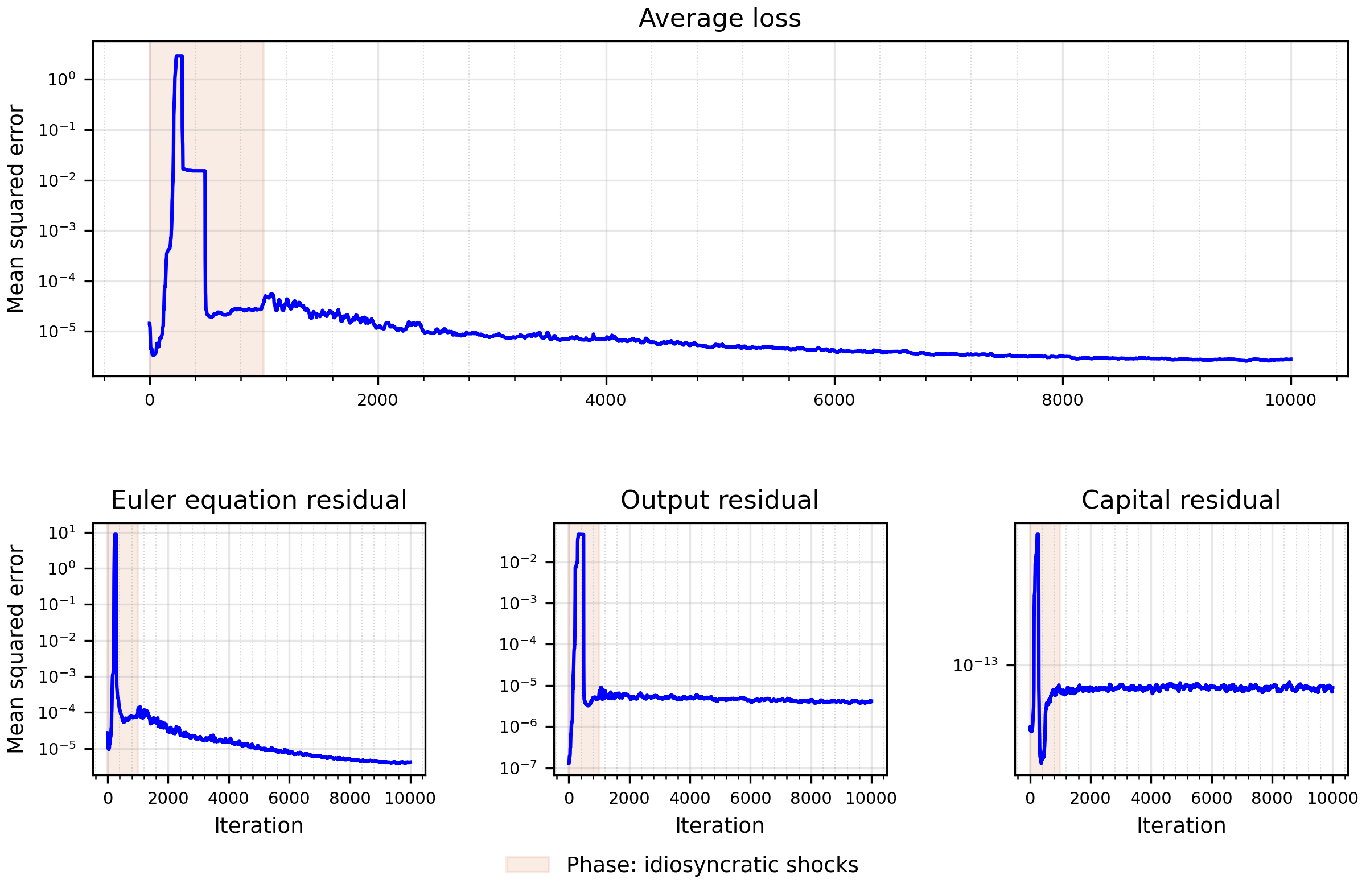
The top panel of the figure below displays the evolution of the average loss over the training. In the lower panels, we plot the in-training evolution of the Euler equation, the output normalization, and the capital consistency condition, which is tracked but not weighted in this stage. To facilitate convergence during training, we gradually introduce idiosyncratic shocks by increasing their variance from a small value to their target levels over the course of the first 1,000 iterations. The red shaded area marks this stage. The training is successful, with clear convergence of the average loss. The breakdown of the loss into the individual residual errors confirms that the neural network learns all policy functions of interest effectively.
The next step is to define a diagnostic to assess how accurate the model solution is after the training of the neural networks has been completed. We use the Euler equation errors, following Judd (1992) and Aruoba et al. (2006). But instead of focusing on one condition, we use the same set of equilibrium conditions used during training, which are the Euler equation and the output normalization,
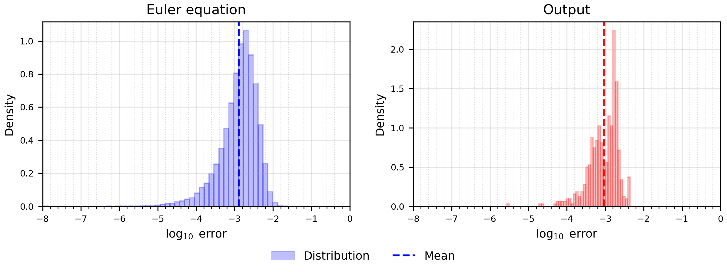
\[err_1=\left|\Psi^{FB}\left(K_t^i-\underline K,\frac{1}{\bar\lambda_t^i}-1\right)\right|,\qquad err_2=\left|Y_t-Y\right|.\]
We simulate 10 economies for 50 periods and calculate the approximation error for each period, drawing 1,000 shocks to evaluate expectations. The replication package uses 1,000 periods. The results of the validation exercise for the two conditions are shown in the figure below. The residual errors are well contained, even in the right tails of the distributions. Each distribution is approximately bell-shaped, with modes close to the dashed lines, which mark the mean \(\log_{10}\) absolute error over the plotted range. Large approximation errors are therefore rare. Moreover, the symmetry and concentration of the distributions around small values further reinforce the reliability of the neural network solution, indicating that the approximation performs consistently well across a wide range of simulated states.
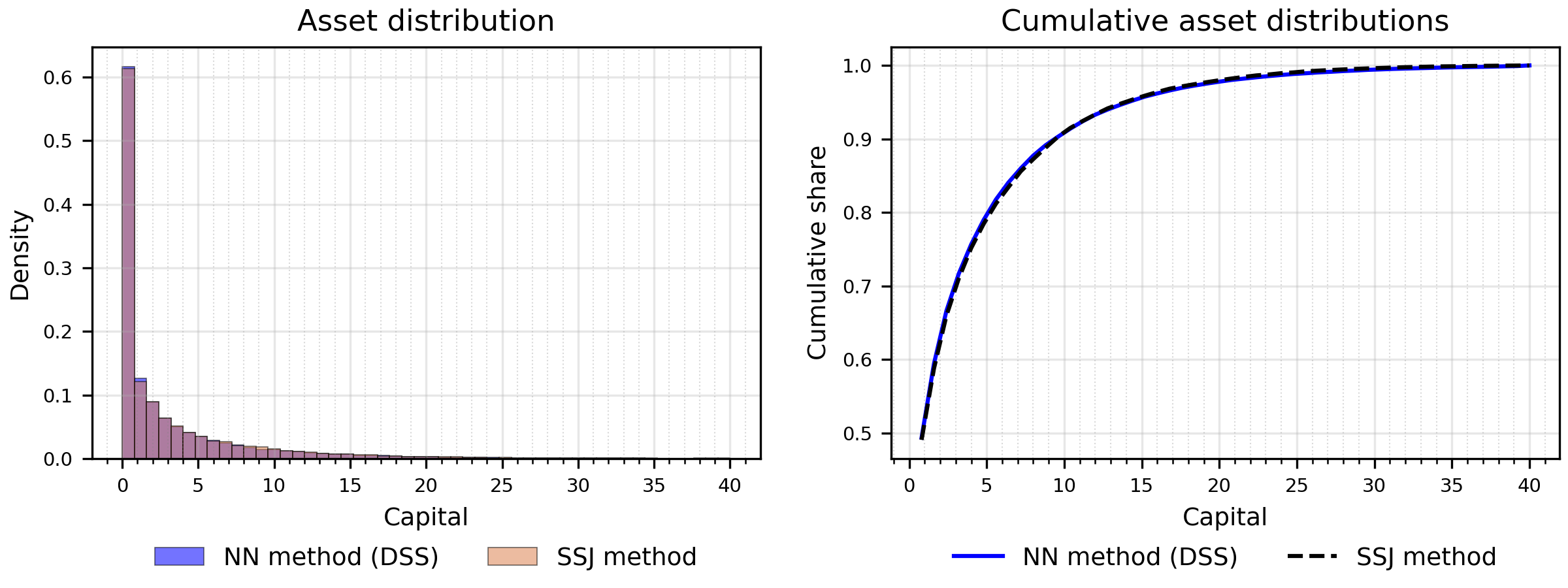
The figure below shows the distribution of capital holdings, with the left panel showing the histogram and the right panel the corresponding cumulative distribution function. Each distribution is obtained by averaging across 500 simulated economies (batches). The lighter bars and the dashed line are the SSJ steady state, which the comparison below discusses.
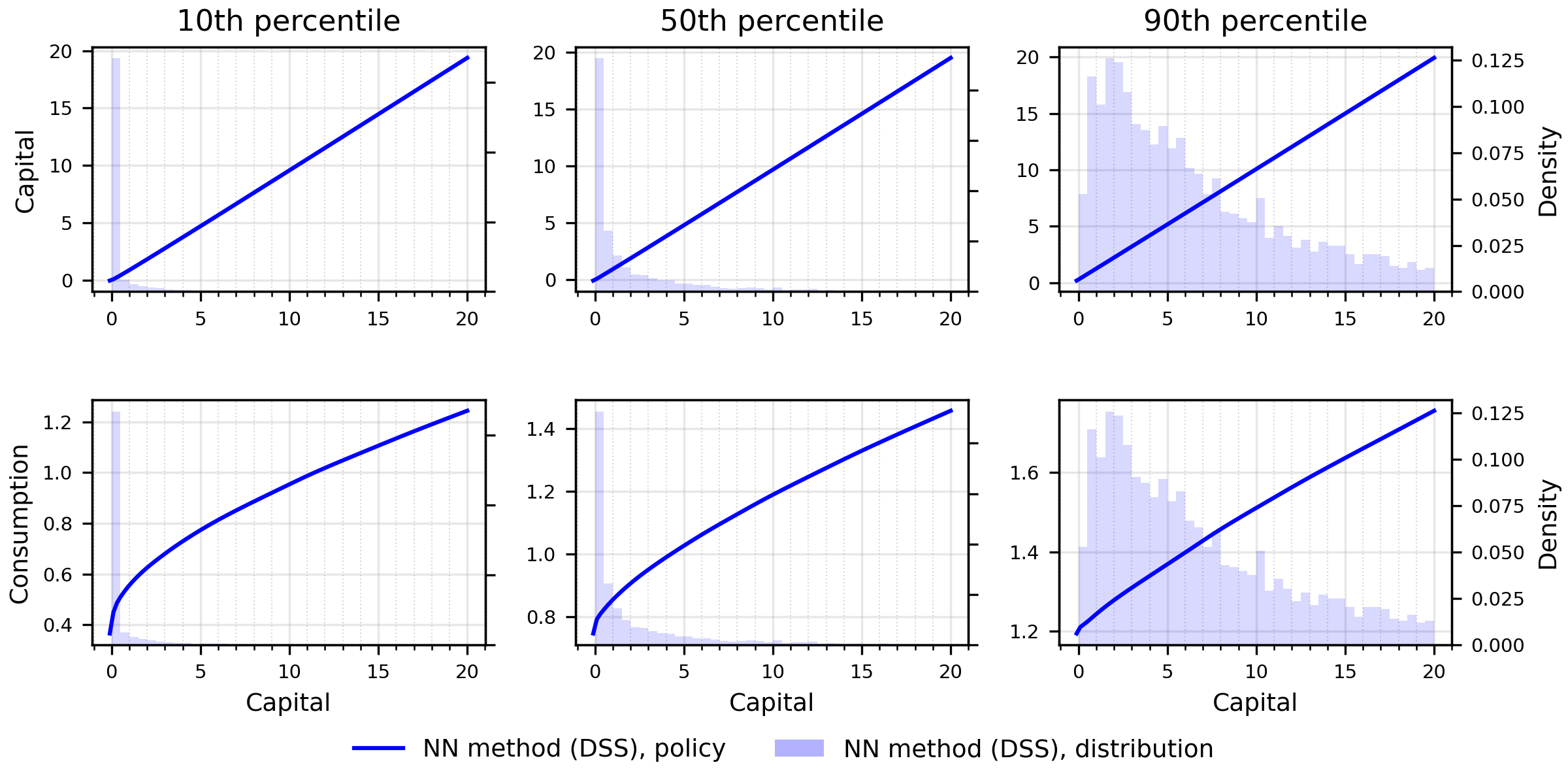
The next figure shows the bar graph of the capital distribution conditional on various levels of productivity (10th percentile, 50th percentile, and 90th percentile) along with the policy functions of capital and consumption.
Full equilibrium
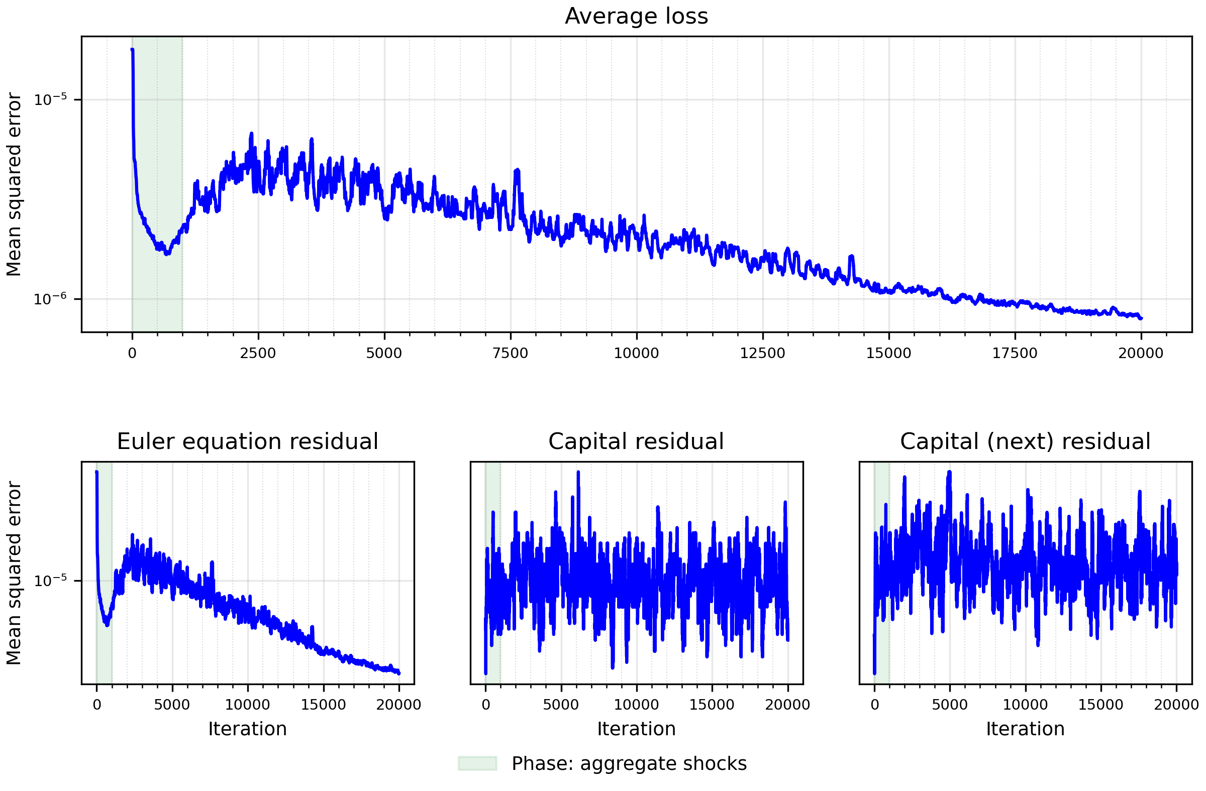
The top panel of the figure below displays the evolution of the average loss over the training for 20,000 iterations. In the other panels, we plot the in-training evolution of the Euler equation and the capital conditions, which are overidentifying restrictions. To facilitate convergence during training, we gradually introduce aggregate risk by increasing its variance from a small value to its target level over the course of the first 1,000 iterations. The shaded area marks this stage. The training is successful, with clear convergence of the average loss.
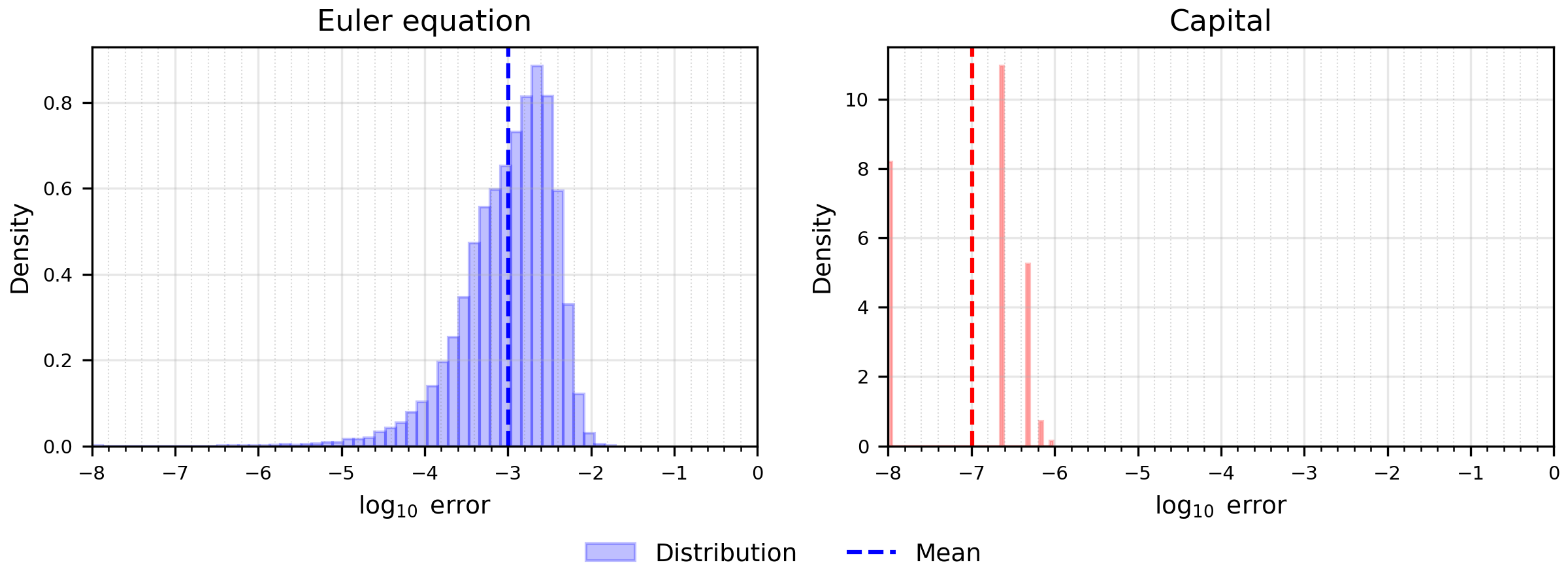
The next step is to calculate the approximation error after the training of the neural networks has been completed. The relevant equation is the absolute error of the Euler equation, \(err_1\) above. We simulate 10 economies for 50 periods with aggregate shocks and calculate the approximation error for each period, drawing 1,000 shocks to evaluate expectations. The results of the validation exercise are shown in the figure below, together with the capital consistency condition. The residual error of the Euler equation is well contained, even in the right tail of the distribution. The distribution is approximately bell-shaped, with the mode close to the dashed line, which marks the mean \(\log_{10}\) absolute error over the plotted range. Large approximation errors are therefore rare. Moreover, the symmetry and concentration of the distribution around small values further reinforce the reliability of the neural network solution, indicating that the approximation performs consistently well across a wide range of simulated states.
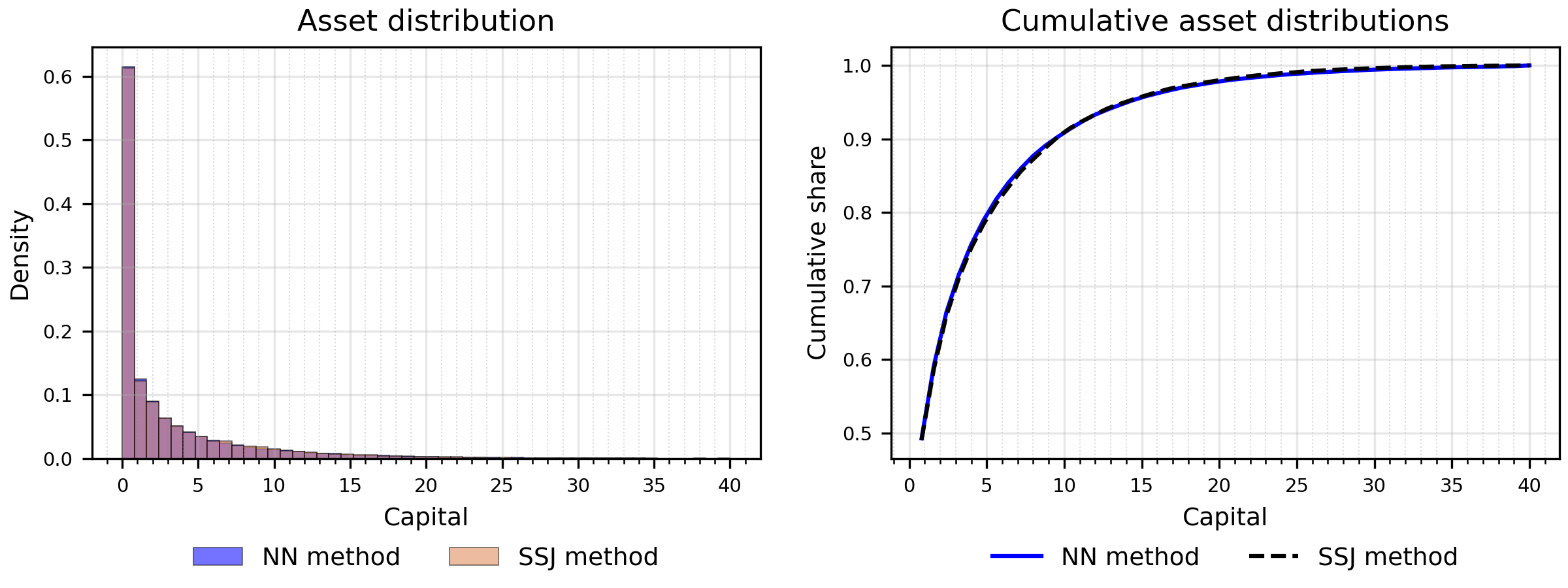
The figure below shows the distribution of capital holdings in the full model, with the left panel showing the histogram and the right panel the corresponding cumulative distribution function. Each distribution is obtained by averaging the stochastic steady state across 500 simulated economies (batches). The impulse responses of the full model are shown in the comparison with the SSJ method below.
Comparison with the sequence-space Jacobian
In the next step, we want to compare our neural network based solution method to a conventional (linear) approach, specifically the sequence-space Jacobian (SSJ) approach of Auclert et al. (2021). We also choose the SSJ due to the availability of their repository, which provides a natural benchmark for scholars and practitioners interested in comparing it with our code. For this comparison, we use the conventional linearized SSJ solution. The solution methods in general do not coincide, as our approach incorporates nonlinear dynamics and aggregate uncertainty affects the equilibrium dynamics. There are also other differences, such as that we do not discretize the shocks. This version of the Krusell–Smith model features only one shock, and therefore aggregate uncertainty does not play a big role in affecting agents’ decisions and equilibrium allocations. Even in its original nonlinear specification, the equilibrium dynamics of aggregate variables in this model remain close to linear, making the solution obtained via the SSJ method a reliable standard for validation. Setting the volatility of aggregate shocks to be very small is problematic, however. Our neural network solver is designed to handle nonlinear models with meaningful aggregate risk, and when aggregate volatility is reduced to negligible levels, the errors become too small to train the networks effectively.
We compare our solution method along the following features: the equilibrium asset distribution, the individual policy functions, and the impulse response functions to the productivity shock.
The full-model asset distribution above compares the capital distribution generated by our method and by the SSJ approach. For our method, we report the distribution at the stochastic steady state, which accounts for the presence of aggregate risk. In contrast, the linearized SSJ solution we use assumes away aggregate uncertainty in the steady state, so its distribution corresponds to the deterministic steady state. Despite this key difference, the two distributions are remarkably similar. Although minor deviations are visible in the tails, the overall shape and key moments align closely, suggesting that our method provides a highly accurate approximation.
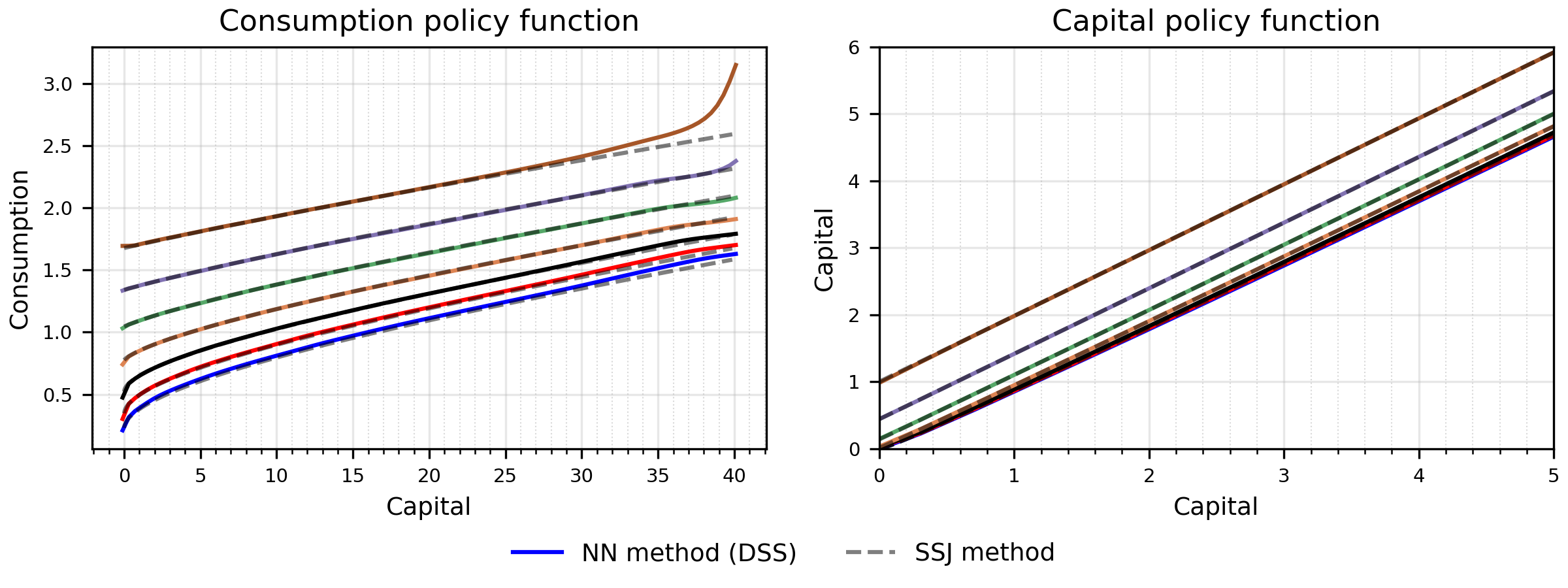
The next step is to compare the two sets of policy functions that determine agents’ consumption and capital decisions, as shown in the figure below. The solid lines depict the policy functions approximated using our method, while the dashed lines correspond to the approximation obtained using the SSJ method. Each color represents one of the seven idiosyncratic labor productivity levels considered in the SSJ, from the least productive agents at the bottom to the most productive ones at the top. We display a shorter horizon for capital for a better visualization.
These seven productivity levels are used solely for the purpose of comparing the results from our solution method with those from SSJ. Our solution method does not rely on discretizing the productivity space. Instead, we treat idiosyncratic labor productivity as the outcome of a continuous AR(1) process, as specified in the model. For the purpose of this comparison, we evaluate the policy functions at the values of the discretization in the code made available by Auclert and coauthors.
Our method successfully replicates the policy functions approximated by the SSJ approach. The largest difference arises for the most productive agents with large asset holdings, who constitute only a very small fraction of the population. As our method imposes an upper bound on the amount of assets that agents can accumulate, these agents increase their consumption to avoid reaching the bound. Increasing the upper bound reduces this effect. Another small discrepancy arises in the behavior of the most productive agents with zero assets, a group that represents an extremely small fraction of agents, and the unproductive agents with large asset holdings. These combinations require highly unlikely sequences of events. Because so few agents follow such a path, the neural network has limited data to learn from, which results in a less accurate approximation of their behavior. Nonetheless, the inaccuracies in these cases are fairly limited, highlighting the strong extrapolative properties of neural networks. Moreover, since these extreme types of agents have almost zero measure in the population, the approximation error introduced by the neural network in this specific region is clearly inconsequential for aggregate outcomes.
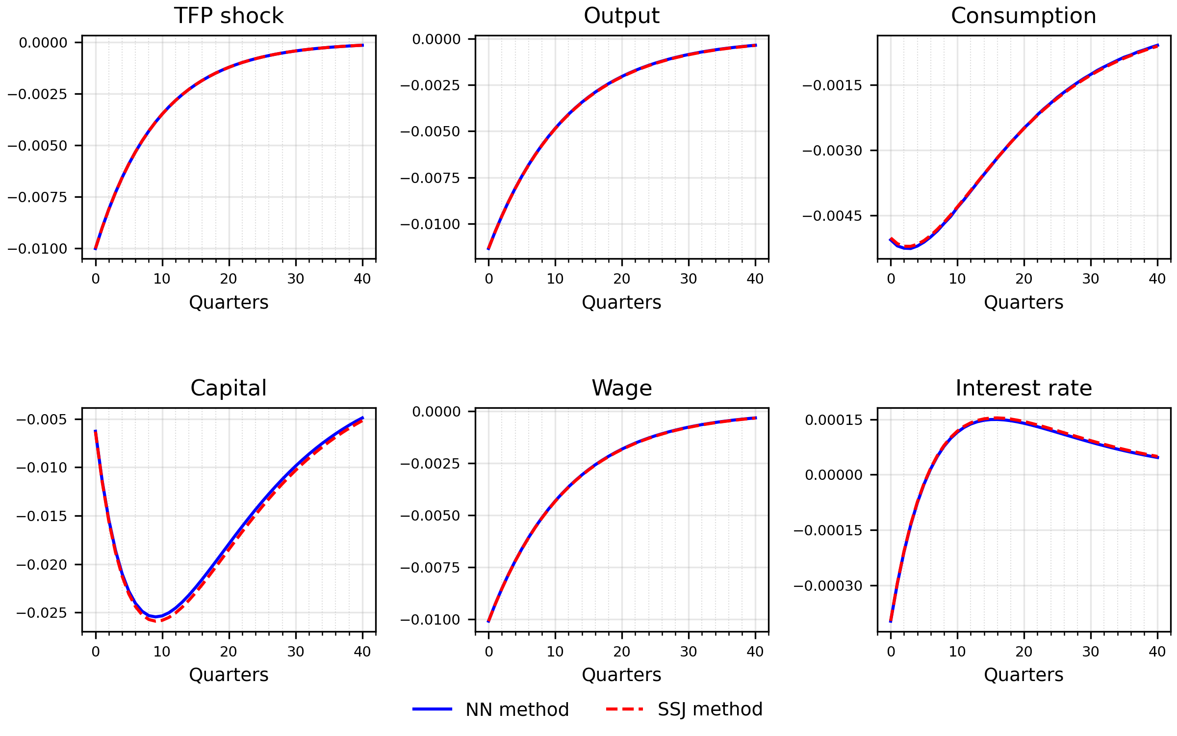
The effects of a TFP shock on the equilibrium dynamics of aggregate variables predicted by the two methods are quite similar, as shown in the figure below. The responses show the deviations from the stochastic steady state (SSS) for the neural network based method. As the SSJ does not feature the SSS, the deviations in that case are shown from the deterministic steady state (DSS). The impulse responses are averaged over 200 simulated economies that share the same idiosyncratic shocks with their unshocked counterparts, so that idiosyncratic shocks of the agents do not affect the results. The transmission of the shock is very similar, as aggregate uncertainty plays only a very limited role.