Krusell–Smith: two assets
We now extend the one-asset heterogeneous agent model by incorporating a second asset. Specifically, households can now also hold government debt. The introduction of the second asset makes the household problem substantially more demanding. Households now choose consumption, capital holdings, and bond holdings, subject to separate optimality conditions and potentially binding lower bounds for both assets. The individual state space is therefore larger, two-dimensional in asset holdings in addition to the idiosyncratic productivity state.
The script coordinates separate model, analysis, and plotting files, as in the paper’s replication package. Its saved networks are the trained networks from that package, so the script reproduces the solution without retraining. Run it from the environment described in Setting up Python.
Model
Households choose consumption \(C_t^i\) to maximize their utility
\[E_0\sum_{t=0}^\infty\beta^t\frac{(C_t^i)^{1-\sigma}}{1-\sigma},\]
with \(\sigma=1\). However, they can now also invest in government bonds, which are bought at the price \(Q_t\) and pay one next period. The budget constraint can be written as
\[C_t^i+K_t^i+Q_tB_t^i+T_t =B_{t-1}^i+(1+r_t)K_{t-1}^i+w_t\bar H\exp(s_t^i),\]
where \(B_t^i\) are the household-specific bond holdings. Holdings away from the bond supply \(B\) carry the cost \(\frac{\gamma}{2}(B_t^i-B)^2\). We assume that each household gets its own cost back as a lump-sum rebate, which it takes as given. The cost and the rebate therefore cancel in the budget constraint, but the marginal cost still enters the bond choice. The agents cannot hold capital or bonds below some limit,
\[K_t^i\geq\underline K,\qquad B_t^i\geq\underline B.\]
The first-order conditions can be written as
\[ \begin{aligned} 1&=\beta\mathbb E_t\left[\left(\frac{C_{t+1}^i}{C_t^i}\right)^{-\sigma}(1+r_{t+1})\right]+\mu_t^i,\\ Q_t+\gamma\left(B_t^i-B\right)&=\beta\mathbb E_t\left[\left(\frac{C_{t+1}^i}{C_t^i}\right)^{-\sigma}\right]+\nu_t^i, \end{aligned} \]
where \(\mu_t^i\) and \(\nu_t^i\) are the normalized Lagrange multipliers on the constraints for individual capital and bond holdings.
The representative firm produces output \(Y_t=A_tK_{t-1}^\alpha N_t^{1-\alpha}\), where total factor productivity follows \(A_{t+1}=(1-\rho_A)A+\rho_AA_t+\sigma_A\epsilon_{t+1}^A\). The first-order conditions are
\[r_t=\alpha\frac{Y_t}{K_{t-1}}-\delta,\qquad w_t=(1-\alpha)\frac{Y_t}{N_t}.\]
The fiscal authority sets taxes \(T_t\) to keep the level of bonds \(B\) constant, \(B=Q_tB+T_t\), so that \(T_t=(1-Q_t)B\) pays for the bond discount. Market clearing for the labor, capital, bond, and goods markets requires
\[N_t=\int\exp(s_t^i)\bar H\,di,\qquad K_t=\int K_t^i\,di,\qquad B=\int B_t^i\,di,\qquad Y_t=\int C_t^i\,di+K_t-(1-\delta)K_{t-1}.\]
Calibration
The calibration follows the one-asset model, with the same discount factor. Productivity, capital, and the bond price of the SSJ steady state are solved so that output is one and the capital and bond markets clear. The additional parameters are the bond supply \(B=1\), which is also the target of the holding cost, the cost \(\gamma=0.025\), and the lower bound \(\underline B=0\). As for capital, bonds have a numerical upper bound \(\overline B=5\), which is checked not to bind after training.
| Parameter | Value | Parameter | Value |
|---|---|---|---|
| Discount factor \(\beta\) | 0.981953 | TFP persistence \(\rho_A\) | 0.9 |
| Risk aversion \(\sigma\) | 1 | TFP innovation SD \(\sigma_A\) | 0.01 |
| Capital share \(\alpha\) | 0.11 | Bond supply \(B\) | 1 |
| Depreciation rate \(\delta\) | 0.025 | Bond holding cost \(\gamma\) | 0.025 |
| Productivity persistence \(\rho_s\) | 0.966 | Lower bounds \(\underline K\), \(\underline B\) | 0, 0 |
| Productivity innovation SD \(\sigma_s\) | 0.129271 | Upper bounds \(\overline K\), \(\overline B\) | 40, 5 |
Neural network solution
Formulation
The state variables and shocks are
\[\mathbb S_t=\left\{\{K_{t-1}^i\}_{i=1}^L,\{B_{t-1}^i\}_{i=1}^L,\{s_t^i\}_{i=1}^L,A_t\right\},\qquad \nu_t=\left\{\{\epsilon_t^{s,i}\}_{i=1}^L,\epsilon_t^A\right\}.\]
All parameters are calibrated in this example,
\[\bar\Theta=\{\beta,\sigma,\alpha,\delta,\rho_s,\sigma_s,\rho_A,\sigma_A,\underline K,\gamma,\underline B,B\}, \qquad\tilde\Theta=\{\}.\]
The individual network \(\psi_{NN}^I\) now solves for consumption and bond holdings,
\[\left\{\begin{pmatrix}C_t^i\\B_t^i\end{pmatrix} =\psi_{NN}^I\left(\mathbb S_t^i,\mathbb S_t,\tilde\Theta\mid\bar\Theta\right)\right\}_{i=1}^L, \qquad\mathbb S_t^i=\{K_{t-1}^i,B_{t-1}^i,s_t^i\}.\]
A steady-state network provides the productivity level and the bond price of the deterministic steady state, \((A,Q)=\psi_{NN}^{SS}(\tilde\Theta\mid\bar\Theta)\), and an aggregate network returns the bond price in the full model, \(Q_t=\psi_{NN}^A(\mathbb S_t,\tilde\Theta\mid\bar\Theta)\). As in the one-asset model, the solution has two stages. The DSS stage trains the household and steady-state networks. The full model then trains a second household network, initialized with the DSS weights, together with the aggregate network, while the steady-state network stays fixed.
The networks have the same architecture as in the one-asset model. Consumption is the representative-agent steady-state level times \(0.2+0.8e^{o}\) of the network output, bonds are the supply times \(-0.2+1.2e^{o}\), and the two steady-state values and the bond price relative to its steady-state level are sigmoids in \([0.8,1.2]\). Capital follows from the budget constraint.
Residuals and loss
Both first-order conditions take the Fischer–Burmeister form of the one-asset model. With \(\bar\lambda_t^i=\beta\mathbb E_t[(C_t^i/C_{t+1}^i)(1+r_{t+1})]\) and \(\bar\psi_t^i=\bigl(\beta\mathbb E_t[C_t^i/C_{t+1}^i]-\gamma(B_t^i-B)\bigr)/Q_t\), the household residuals are
\[F^{1,i}_t=\Psi^{FB}\left(K_t^i-\underline K,\frac{1}{\bar\lambda_t^i}-1\right),\qquad F^{2,i}_t=\Psi^{FB}\left(B_t^i-\underline B,\frac{1}{\bar\psi_t^i}-1\right),\]
each switching to the upper-bound form in the top fifth of its asset range. The first condition governs the optimal choice of capital, while the second governs the optimal choice of government bonds. In the DSS stage, \(F^3=Y_t-1\) normalizes output, \(F^4\) is capital consistency, which is tracked but unweighted there, and \(F^5\) is bond market clearing, \(B-\frac1L\sum_iB_t^i\). In the full model, \(F^3\) and \(F^4\) are capital consistency today and next period and \(F^5\) is bond market clearing. The loss is the weighted mean of the squared residuals over the batch, with the household residuals averaged over the \(L\) households and the next-period residual over the \(M\) shock draws, as in the one-asset model. The weights are \((1,1,1,0,1)\) in the DSS stage and all one in the full model.
Training
The training settings are those of the one-asset model. Each iteration takes 20 internal updates on a batch of \(N_{batch}=100\) economies with \(M=50\) antithetic draws. The DSS stage runs 10,000 iterations and the full model 20,000, with AdamW, a learning-rate warmup to \(10^{-4}\) followed by cosine annealing to \(10^{-8}\), and the same shock phase-ins, simulation steps, and panel resets. An economy is also reset when its bond holdings leave their bounds.
In the code
Set the parameters and shocks
The household, technology, and bond parameters are read from the SSJ reference. ranges is empty, because no parameter varies during training.
examples/kstwo/kstwo.py
parameters = {
    # Household and technology, from the SSJ calibration.
    "beta": ref_ss["beta"],
    "delta": ref_ss["delta"],
    "alpha": ref_ss["alpha"],
    "rho_s": ref_ss["rho_e"],
    "sigma_s": ref_ss["sd_e"] * math.sqrt(1 - ref_ss["rho_e"] ** 2),
    # Aggregate productivity shock.
    "rho_A": 0.9,
    "sigma_A": 0.01,
    # Bounds on capital.
    "k_bar": 0.0,
    "k_down": 40.0,
    # Bond: holding cost, bounds, and supply.
    "gamma": ref_ss["gamma"],
    "b_bar": 0.0,
    "b_down": 5.0,
    "B": ref_ss["B"],
}

ranges = {}  # No parameter varies during training.

shocks_ind = {"s": torch.distributions.Normal(0.0, 1.0)}

shocks_agg = {"A_scale": torch.distributions.Normal(0.0, 1.0)}The code names map to the symbols above as follows.
| Code | Symbol | Meaning |
|---|---|---|
k, b |
\(K_t^i\), \(B_t^i\) | capital and bonds |
s |
\(s_t^i\) | log productivity |
k_bar, k_down, b_bar, b_down |
\(\underline K\), \(\overline K\), \(\underline B\), \(\overline B\) | bounds on the assets |
B, gamma |
\(B\), \(\gamma\) | bond supply and holding cost |
Q, Q_dss |
\(Q_t\), \(Q\) | bond price and its steady-state level |
T |
\(T_t\) | lump-sum tax |
A_scale, Kl |
\(A_t-A_{RA}\), \(K_{t-1}\) | aggregate state |
A_dss |
\(A\) | steady-state productivity, learned by the DSS network |
lambda_comp, psi_comp |
\(\bar\lambda_t^i\), \(\bar\psi_t^i\) | expected terms of the capital and bond conditions |
res_fb_k, res_fb_b |
\(F^1\), \(F^2\) | household residuals for capital and bonds |
res_y, res_k, res_k_next |
\(F^3\), \(F^4\) | output normalization (DSS) and capital consistency today and next period |
res_b |
\(F^5\) | bond market clearing |
_ind, _dist suffixes |
the \(L\)-household panel and the distribution panel |
Evaluate and transform policies
hh_policy evaluates the household network through _hh_choices, which returns consumption relative to its steady-state level and bonds relative to the supply. agg_policy returns the bond price relative to its steady-state level, and dss_policy the steady-state productivity level and bond price.
examples/kstwo/kstwo_model.py
def _hh_choices(self, network, state_ind, state_dist, state_agg, par, mc=None):
    """Household consumption relative to steady-state consumption (above 0.2) and bond
    holdings relative to the bond supply (above -0.2)."""
    hh_output = network(**self._state_inputs(state_dist, state_agg, mc=mc, state_ind=state_ind),
                        par=self._prepare_par_input(par=par, mc=mc))
    c_scale = 0.2 + torch.exp(hh_output[..., 0:1]) / (1.0 / (1 - 0.2))
    b_scale = -0.2 + torch.exp(hh_output[..., 1:2]) / (1.0 / (1 + 0.2))
    return c_scale, b_scale

def hh_policy(self, state_ind, state_dist, state_agg, par, mc=None):
    return self._hh_choices(self.hh_network, state_ind, state_dist, state_agg, par, mc=mc)

def agg_policy(self, state_dist, state_agg, par, mc=None):
    """Bond price relative to its DSS level, in [0.8, 1.2]."""
    agg_output = self.agg_network(**self._state_inputs(state_dist, state_agg, mc=mc),
                                  par=self._prepare_par_input(par=par, mc=mc))
    return 0.8 + torch.sigmoid(agg_output[..., 0:1]) * (1.2 - 0.8)

def dss_policy(self, par, mc=None):
    """DSS productivity level relative to the steady-state level and DSS bond price, both in
    [0.8, 1.2]."""
    dss_output = self.dss_network(par=self._prepare_par_input(par=par, mc=mc))
    A_dss_scale = 0.8 + torch.sigmoid(dss_output[..., 0:1]) * (1.2 - 0.8)
    Q_dss = 0.8 + torch.sigmoid(dss_output[..., 1:2]) * (1.2 - 0.8)
return A_dss_scale, Q_dssForm the equilibrium errors
The method below evaluates current consumption and bonds for both panels, computes factor prices, the tax, and each household’s capital from the budget constraint, and advances the states with the shock draws in e. It then evaluates future policies and the future bond price, averages over the draws, and forms the five residuals.
examples/kstwo/kstwo_model.py
def residuals(self, e, mc, detach_next=True, scale_ind=1, scale_agg=1):
    par, ss = self.par_draw, self.ss
    state_ind, state_dist, state_agg = self.state_ind, self.state_dist, self.state_agg

    c_ind_scale, b_ind_scale = self.hh_policy(state_ind, state_dist, state_agg, par)
    c_ind = c_ind_scale * ss.C
    b_ind = b_ind_scale * par.B
    c_dist_scale, b_dist_scale = self.hh_policy(state_dist, state_dist, state_agg, par)
    c_dist = c_dist_scale * ss.C
    b_dist = b_dist_scale * par.B
    A_dss_scale, Q_dss = self.dss_policy(par)
    A_dss = A_dss_scale * ss.A
    Q = self.agg_policy(state_dist, state_agg, par) * Q_dss
    A = state_agg.A_scale + ss.A

    C = torch.mean(c_dist, dim=-2, keepdim=True)
    Kl = state_agg.Kl
    N = ss.N * torch.mean(torch.exp(state_dist.s), dim=-2, keepdim=True)
    Y, r, w = self.factor_prices(A, Kl, N, par)
    T = (1 - Q) * par.B          # lump-sum tax that finances the bond discount

    # Budget constraint
    k_ind = (1 + r) * state_ind.k + state_ind.b + w * torch.exp(state_ind.s) * ss.N - Q * b_ind - c_ind - T
    k_dist = (1 + r) * state_dist.k + state_dist.b + w * torch.exp(state_dist.s) * ss.N - Q * b_dist - c_dist - T

    K = Y - C + (1 - par.delta) * Kl

    # Next period
    shape_ind = e["shocks_ind"].s.shape
    shape_dist = e["shocks_dist"].s.shape
    shape_agg = e["shocks_agg"].A_scale.shape

    s_ind_next = self._ar1_next(state_ind.s, e["shocks_ind"].s, par, scale_ind)
    s_dist_next = self._ar1_next(state_dist.s, e["shocks_dist"].s, par, scale_ind)
    A_next = (1 - par.rho_A) * A_dss + par.rho_A * (state_agg.A_scale + ss.A) + e["shocks_agg"].A_scale * par.sigma_A * scale_agg

    state_ind_next = State({"k": k_ind.expand(shape_ind), "b": b_ind.expand(shape_ind), "s": s_ind_next})
    state_dist_next = State({"k": k_dist.expand(shape_dist), "b": b_dist.expand(shape_dist), "s": s_dist_next})
    state_agg_next = State({"A_scale": A_next - ss.A, "Kl": K.expand(shape_agg)})

    with torch.set_grad_enabled(not detach_next):
        c_ind_scale_next, _ = self.hh_policy(state_ind_next, state_dist_next, state_agg_next, par, mc=mc)
        c_dist_scale_next, b_dist_scale_next = self.hh_policy(state_dist_next, state_dist_next, state_agg_next, par, mc=mc)
        Q_scale_next = self.agg_policy(state_dist_next, state_agg_next, par, mc=mc)
    c_ind_next = c_ind_scale_next * ss.C
    c_dist_next = c_dist_scale_next * ss.C
    b_dist_next = b_dist_scale_next * par.B
    Q_next = Q_scale_next * Q_dss

    C_next = torch.mean(c_dist_next, dim=-2, keepdim=True)
    N_next = ss.N * torch.mean(torch.exp(state_dist_next.s), dim=-2, keepdim=True)
    Y_next, r_next, w_next = self.factor_prices(A_next, K, N_next, par)
    T_next = (1 - Q_next) * par.B

    # Expected discounted returns (log utility); gamma * (b - B) is the marginal holding cost of bonds
    q = par.beta * (c_ind_next / c_ind) ** (-1)
    lambda_comp = torch.mean(q * (r_next + 1), dim=0)
    psi_comp = (torch.mean(q, dim=0) - par.gamma * (b_ind - par.B)) / Q

    k_dist_next = (1 + r_next) * state_dist_next.k + state_dist_next.b + w_next * torch.exp(state_dist_next.s) * ss.N - Q_next * b_dist_next - T_next - c_dist_next
    K_next = Y_next - C_next + (1 - par.delta) * K

    R_fb_k = self._fb_bounds(k_ind, par.k_bar, par.k_down, lambda_comp)
    R_fb_b = self._fb_bounds(b_ind, par.b_bar, par.b_down, psi_comp)
    R_k = K - torch.mean(k_dist, dim=-2, keepdim=True)
    R_k_next = K_next - torch.mean(k_dist_next, dim=-2, keepdim=True)
    R_b = par.B - torch.mean(b_dist, dim=-2, keepdim=True)

return [R_fb_k, R_fb_b, R_k, R_k_next, R_b]The DSS version has the same structure, with the learned steady-state productivity level and bond price in place of the stochastic ones.
examples/kstwo/kstwo_model.py
def dss_residuals(self, e, mc, detach_next=True, scale_ind=1, scale_agg=0):
    par, ss = self.par_draw, self.ss
    state_ind, state_dist, state_agg = self.state_ind, self.state_dist, self.state_agg

    c_ind_scale, b_ind_scale = self.dss_hh_policy(state_ind, state_dist, state_agg, par)
    c_ind = c_ind_scale * ss.C
    b_ind = b_ind_scale * par.B
    c_dist_scale, b_dist_scale = self.dss_hh_policy(state_dist, state_dist, state_agg, par)
    c_dist = c_dist_scale * ss.C
    b_dist = b_dist_scale * par.B
    A_dss_scale, Q_dss = self.dss_policy(par)
    A_dss = A_dss_scale * ss.A

    C = torch.mean(c_dist, dim=-2, keepdim=True)
    Kl = state_agg.Kl
    N = ss.N * torch.mean(torch.exp(state_dist.s), dim=-2, keepdim=True)
    Y, r, w = self.factor_prices(A_dss, Kl, N, par)
    T = (1 - Q_dss) * par.B      # lump-sum tax that finances the bond discount
    K = Y - C + (1 - par.delta) * Kl

    # Budget constraint
    k_ind = (1 + r) * state_ind.k + state_ind.b + w * torch.exp(state_ind.s) * ss.N - Q_dss * b_ind - c_ind - T
    k_dist = (1 + r) * state_dist.k + state_dist.b + w * torch.exp(state_dist.s) * ss.N - Q_dss * b_dist - c_dist - T

    # Next period
    shape_ind = e["shocks_ind"].s.shape
    shape_dist = e["shocks_dist"].s.shape
    shape_agg = e["shocks_agg"].A_scale.shape

    s_ind_next = self._ar1_next(state_ind.s, e["shocks_ind"].s, par, scale_ind)
    s_dist_next = self._ar1_next(state_dist.s, e["shocks_dist"].s, par, scale_ind)
    A_next = (1 - par.rho_A) * A_dss + par.rho_A * (state_agg.A_scale + ss.A) + e["shocks_agg"].A_scale * par.sigma_A * scale_agg

    state_ind_next = State({"k": k_ind.expand(shape_ind), "b": b_ind.expand(shape_ind), "s": s_ind_next})
    state_dist_next = State({"k": k_dist.expand(shape_dist), "b": b_dist.expand(shape_dist), "s": s_dist_next})
    state_agg_next = State({"A_scale": A_next - ss.A, "Kl": K.expand(shape_agg)})

    with torch.set_grad_enabled(not detach_next):
        c_ind_scale_next, _ = self.dss_hh_policy(state_ind_next, state_dist_next, state_agg_next, par, mc=mc)
    c_ind_next = c_ind_scale_next * ss.C

    N_next = ss.N * torch.mean(torch.exp(state_dist_next.s), dim=-2, keepdim=True)
    _, r_next, _ = self.factor_prices(A_dss, K, N_next, par)

    # Expected discounted returns (log utility); gamma * (b - B) is the marginal holding cost of bonds
    q = par.beta * (c_ind_next / c_ind) ** (-1)
    lambda_comp = torch.mean(q * (r_next + 1), dim=0)
    psi_comp = (torch.mean(q, dim=0) - par.gamma * (b_ind - par.B)) / Q_dss

    R_fb_k = self._fb_bounds(k_ind, par.k_bar, par.k_down, lambda_comp)
    R_fb_b = self._fb_bounds(b_ind, par.b_bar, par.b_down, psi_comp)
    R_y = Y - ss.Y
    R_k = K - torch.mean(k_dist, dim=-2, keepdim=True)
    R_b = par.B - torch.mean(b_dist, dim=-2, keepdim=True)

return [R_fb_k, R_fb_b, R_y, R_k, R_b]loss adds the weighted mean squared residuals into the training loss. It also returns each unweighted equation loss for the loss plots.
examples/kstwo/kstwo_model.py
def loss(self, residuals, criterion, names, weights=None):
    """Weighted sum of per-residual MSEs (the scalar to backprop) plus the unweighted per-residual components for logging."""
    if weights is None:
        weights = [1.0] * len(residuals)
    loss = [weights[i] * criterion(r, target=torch.zeros_like(r)) for i, r in enumerate(residuals)]
    with torch.no_grad():
        loss_components = {name: torch.mean(r ** 2) for name, r in zip(names, residuals)}
return sum(loss), loss_componentsTrain in two stages
The repository ships the trained networks from the replication package. Leave load_dss and load_full set to True to load them. Set load_full = False to retrain the full model, and also set load_dss = False to solve the DSS again. Between the two stages, warm_start_full copies the DSS household weights into the full model’s household network.
The computations are performed on an NVIDIA GeForce RTX 5090 GPU with 32 GB of memory. The computational time is around 29 minutes for the DSS and 86 minutes for the full equilibrium. Training takes far longer on a CPU.
The two stages share the training loop. They differ in the number of iterations, the AdamW epsilon, and the equation weights, and the full stage skips the extra simulation steps after a parameter redraw (redraw_steps=0).
examples/kstwo/kstwo.py
# The DSS stage tracks capital consistency but gives it no weight.
dss_config = TrainingConfig(
    iteration=10000,
    internal=20,
    batch=100,
    mc=50,
    lr=1e-4,
    adam_eps=1e-8,
    weights=ConstantWeights(weights=[1.0, 1.0, 1.0, 0.0, 1.0]),
    device=DEVICE,
    seed=1234,
)

full_config = TrainingConfig(
    iteration=20000,
    internal=20,
    batch=100,
    mc=50,
    lr=1e-4,
    adam_eps=1e-10,
    redraw_steps=0,
    weights=ConstantWeights(weights=[1.0] * model.N_RESIDUALS),
    device=DEVICE,
    seed=1234,
)
examples/kstwo/kstwo.py
dss_path = networks / "dss.pt"
full_path = networks / "full.pt"
train_full = not load_full or not full_path.exists()
train_dss = train_full and (not load_dss or not dss_path.exists())

if train_dss:
    print("Training the deterministic steady state...")
    model.train_dss_model(dss_config)
    model.save(networks, name="dss")
    # A new DSS needs a new full model, so delete the saved one.
    full_path.unlink(missing_ok=True)
elif train_full:
    print("Loading the deterministic steady state.")
    model.load(dss_path)
examples/kstwo/kstwo.py
if train_full:
    print("Training the model with aggregate risk...")
    model.warm_start_full()
    model.train_model(full_config)
    model.save(networks, name="full")
else:
    print("Loading the model with aggregate risk.")
model.load(full_path)Results
The analysis uses the methods of the replication package with smaller samples, so it runs on a CPU in about 10 minutes. It compares with the SSJ reference shipped in examples/kstwo/outputs/reference. The results are saved and reused. Set load_analysis = False to recompute them.
Deterministic steady state
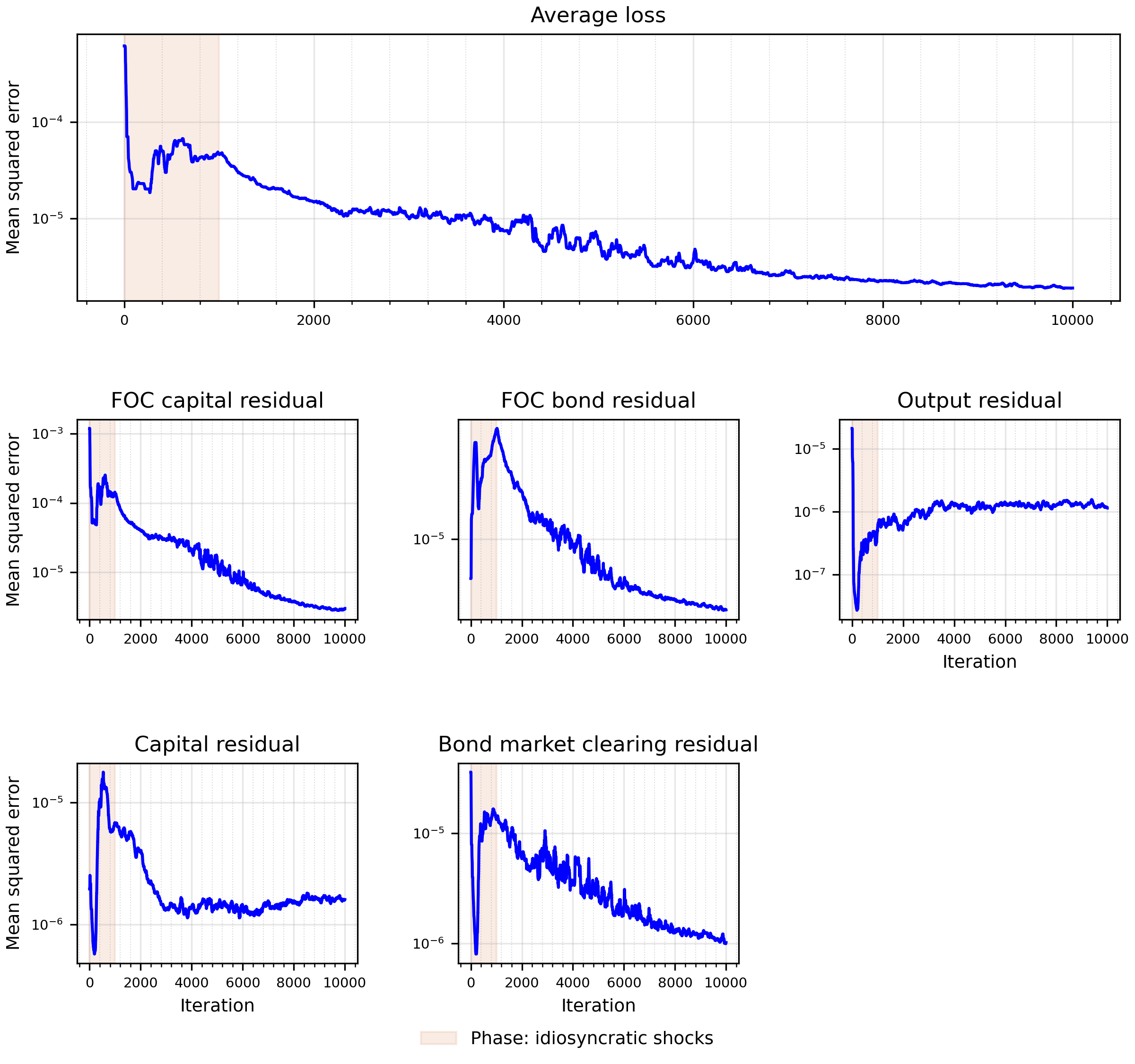
The figure below displays the evolution of the average loss over the training, with the individual conditions below it. As before, we gradually introduce idiosyncratic shocks, as marked by the red shaded area.
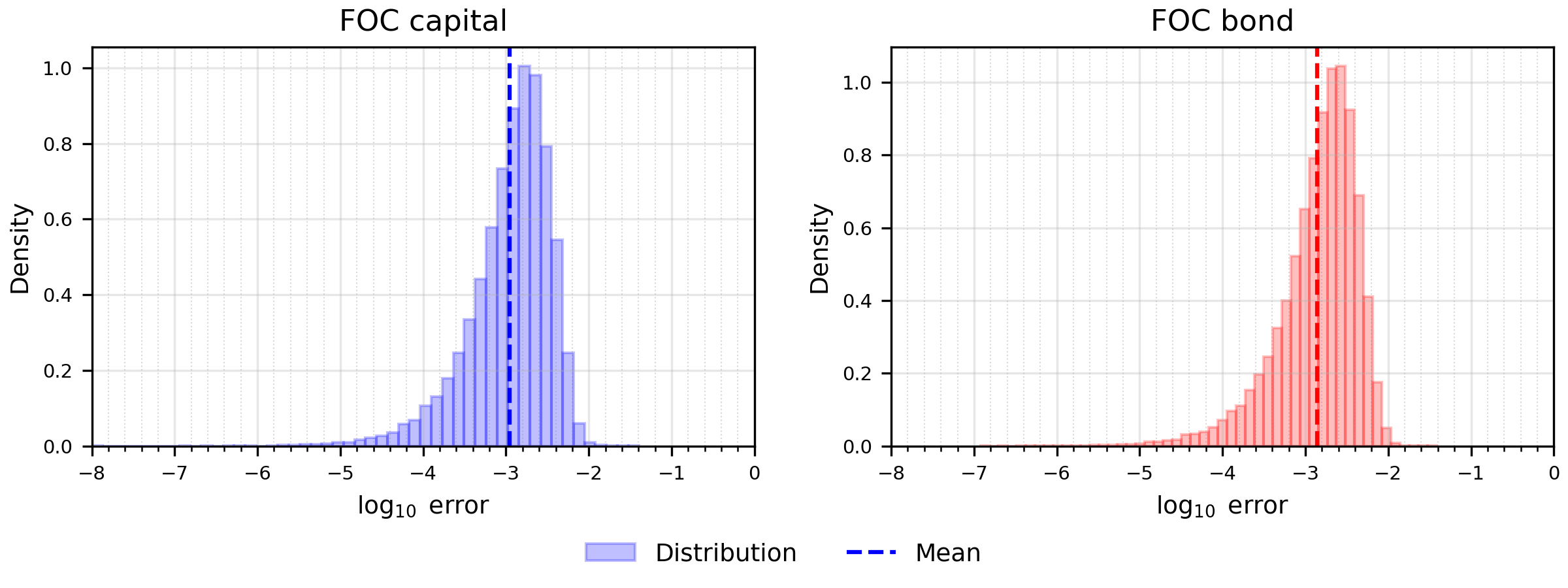
Because the household problem now involves two asset choices, we focus our diagnostics on the errors in the first-order conditions for capital and bonds. These conditions are more demanding than in the one-asset model because the neural network must jointly learn the household’s optimal allocation across the two assets. We consider the absolute errors in the two complementarity conditions,
\[err_1=\left|\Psi^{FB}\left(K_t^i-\underline K,\frac{1}{\bar\lambda_t^i}-1\right)\right|,\qquad err_2=\left|\Psi^{FB}\left(B_t^i-\underline B,\frac{1}{\bar\psi_t^i}-1\right)\right|.\]
The first condition governs the optimal choice of capital, while the second governs the optimal choice of government bonds. The Fischer–Burmeister function \(\Psi^{FB}\) writes each occasionally binding lower-bound condition as a single equation that the networks can be trained on.
We simulate 10 economies for 50 periods and calculate the approximation error for each period, drawing 1,000 shocks to evaluate expectations. The replication package uses 1,000 periods. The figure below reports the distributions of these post-training approximation errors. The residual errors remain well contained in this more elaborate two-asset environment, including in the right tails of the distributions. Both distributions are approximately bell-shaped, with most observations concentrated around the corresponding mean absolute errors. Large approximation errors are therefore rare and are unlikely to systematically affect the model’s dynamics.
Importantly, the approximation error in the first-order condition for capital is virtually the same as in the one-asset model. The mean post-training error is close to \(-3\) in \(\log_{10}\) units in both cases, and the two distributions have very similar shapes. Thus, adding a second asset does not materially reduce the accuracy with which the neural network solves the capital-choice problem. At the same time, the small errors in the bond condition show that the neural network method can accurately learn the additional portfolio margin introduced by the second asset.
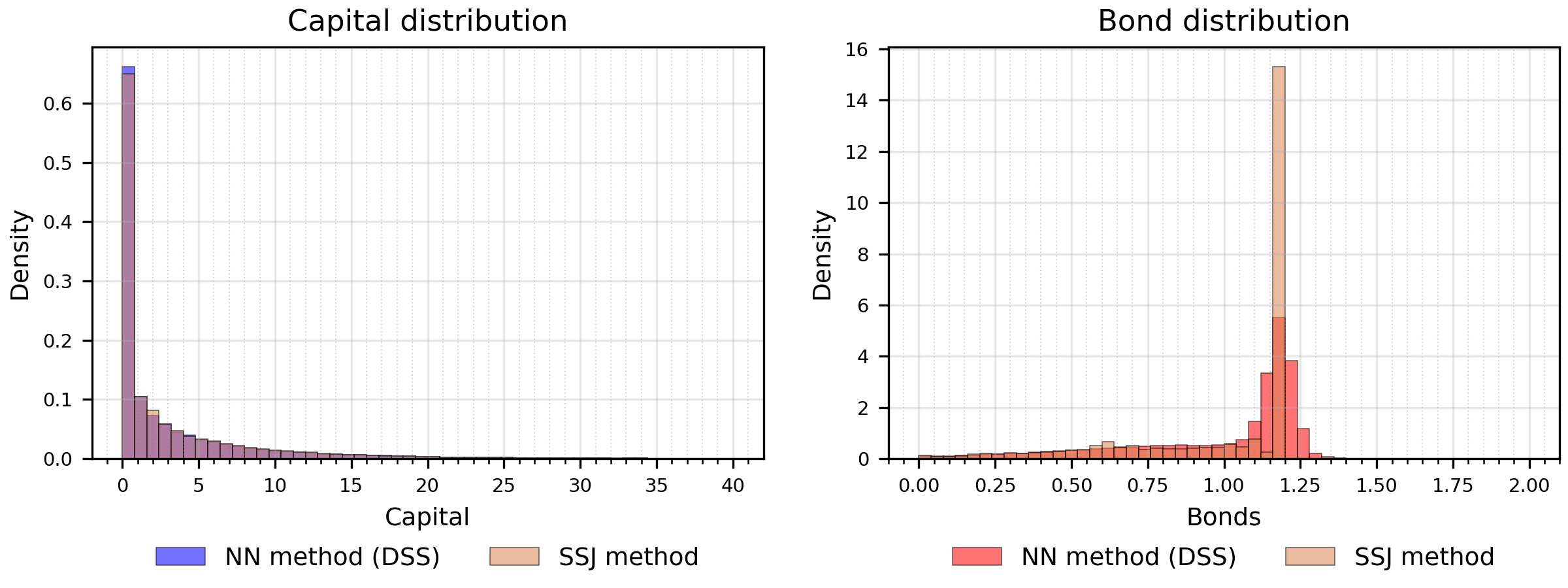
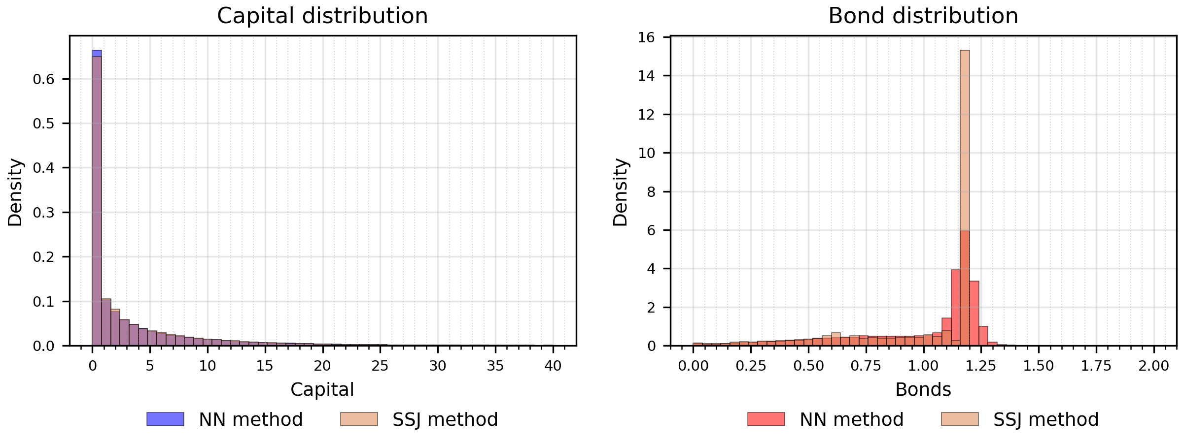
The figure below shows the distribution of capital and bond holdings, with the left panel showing the histogram for capital and the right panel the corresponding histogram for bonds. Each distribution is obtained by averaging across 500 simulated economies (batches). The lighter bars are the SSJ steady state.
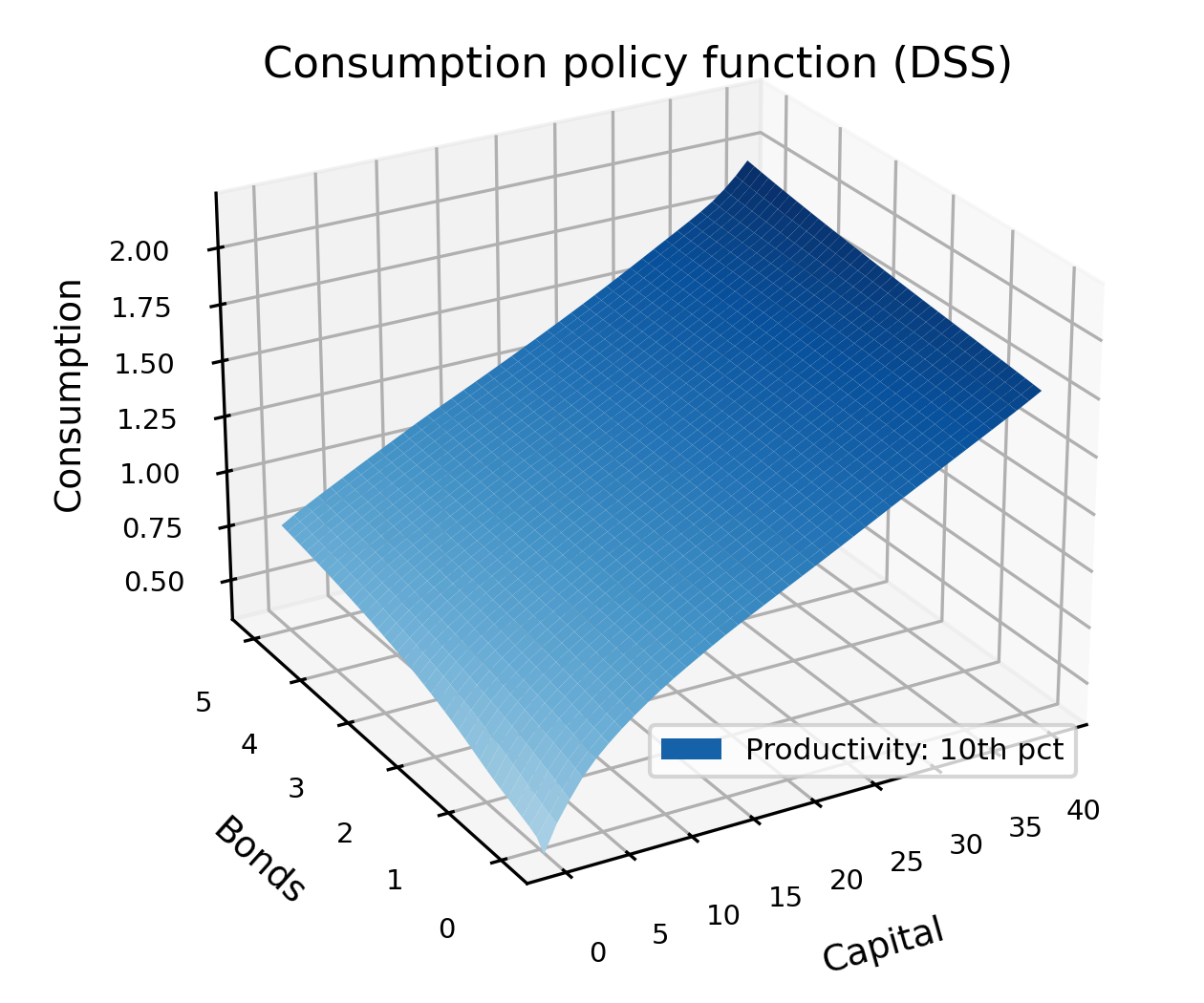
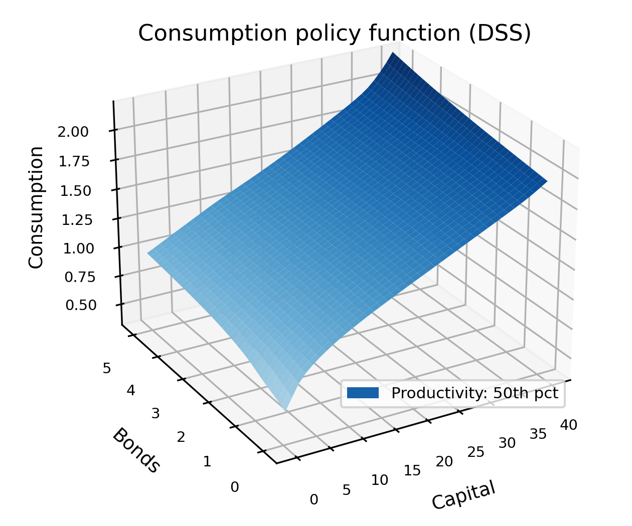
The next figures report the individual consumption policy function over different combinations of capital and bond holdings. The first evaluates the policy function at the 10th percentile of the productivity distribution, while the second evaluates it at the 50th percentile. These figures provide a direct illustration of the richer household problem. Consumption is now a function of two endogenous asset positions rather than a single wealth variable. The neural network must therefore learn how consumption varies jointly with capital and bonds and with idiosyncratic productivity.
The smoothness and economically coherent shape of the estimated policy functions provide an additional diagnostic of the quality of the solution. Consumption rises with household resources, while its sensitivity to either asset depends on the household’s position in the joint asset distribution and on its productivity state. The script also compares the DSS policies over capital with the SSJ policies at its seven productivity levels, for a household that holds the bond supply.
Full equilibrium
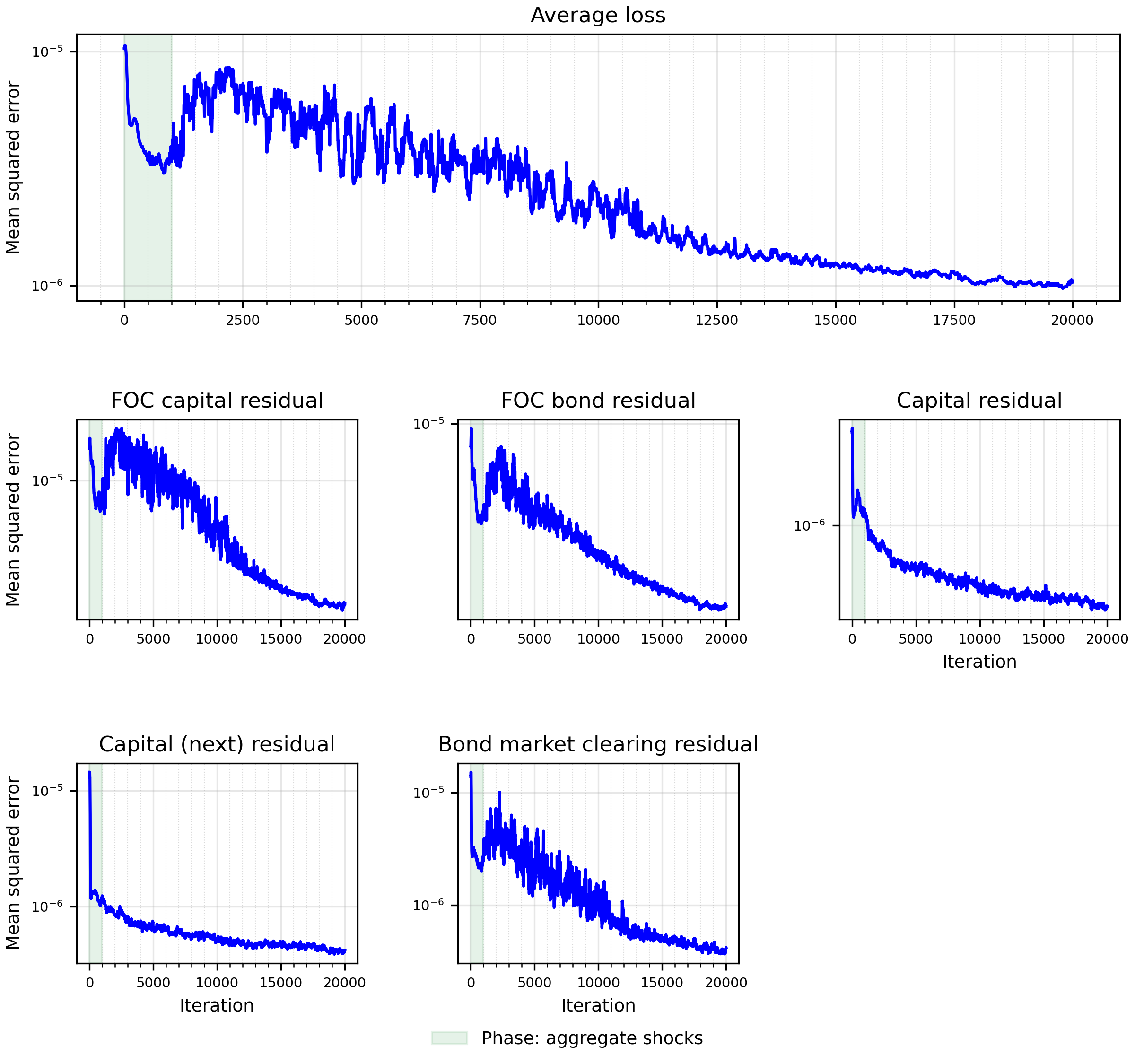
The figure below displays the evolution of the average loss over 20,000 training iterations, with the individual conditions below it. To facilitate convergence, we gradually introduce aggregate risk by increasing the variance of the aggregate shock from a small initial value to its calibrated level over the first 1,000 iterations. The shaded area marks the period during which aggregate risk is scaled up. The average loss declines and converges, indicating that the neural network successfully learns the full-equilibrium solution.
We then evaluate the approximation errors after the training of the neural networks is complete. As in the deterministic steady state, the relevant diagnostics are the absolute errors in the first-order conditions for capital and bonds. We simulate 10 economies for 50 periods with aggregate shocks and compute the approximation errors in each period, using 1,000 Monte Carlo draws to evaluate the expectations entering the household optimality conditions.
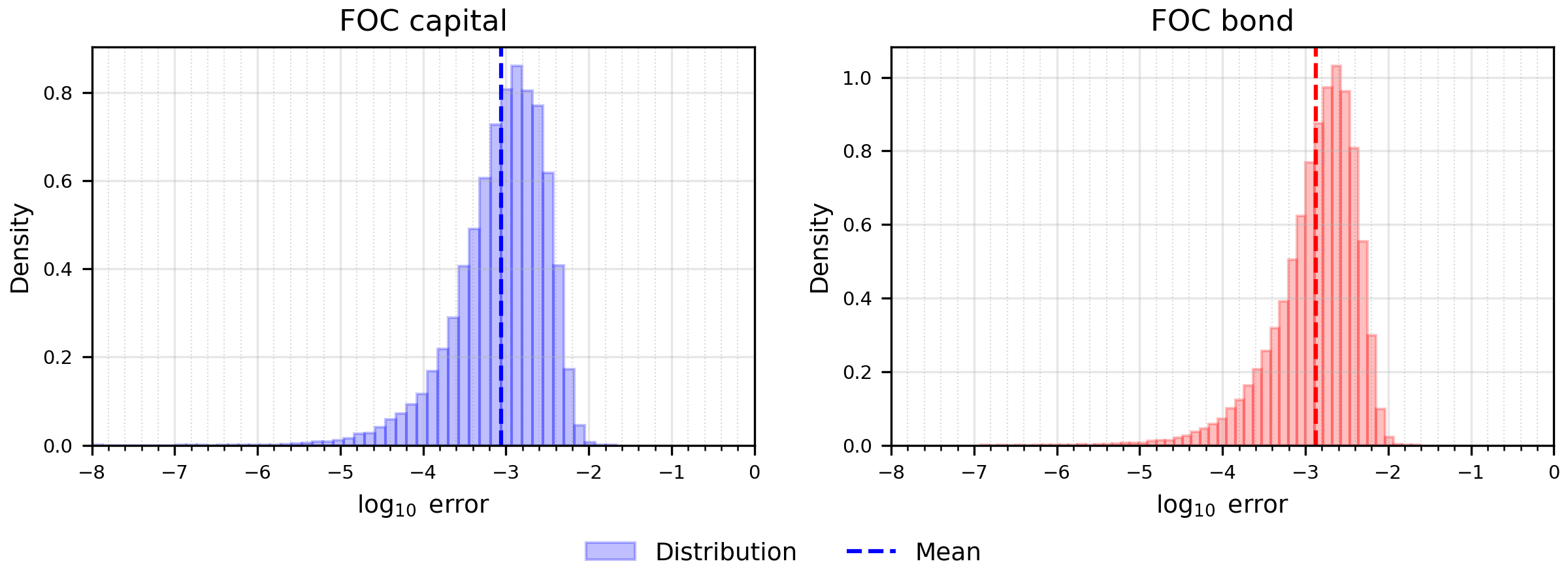
The figure below reports the resulting distributions. The residual errors in both conditions remain well contained, including in the right tails. The distributions are approximately bell-shaped, with their modes close to the dashed lines, which mark the mean \(\log_{10}\) absolute error over the plotted range. Large errors are therefore rare. Importantly, the approximation error for the capital condition is comparable to that obtained in the one-asset model. In both cases, the mean post-training approximation error is close to \(-3\) in \(\log_{10}\) units, and the shapes of the error distributions are very similar. In sum, although introducing a second asset materially increases the dimensionality and complexity of the household problem, the approximation diagnostics remain very well behaved, underscoring the reliability of our method.
The figure below shows the distribution of asset holdings in the full model, with the left panel showing the histogram for capital and the right panel the histogram for bonds. Each distribution is obtained by averaging the stochastic steady state across 500 simulated economies (batches). The lighter bars are the SSJ deterministic steady state.
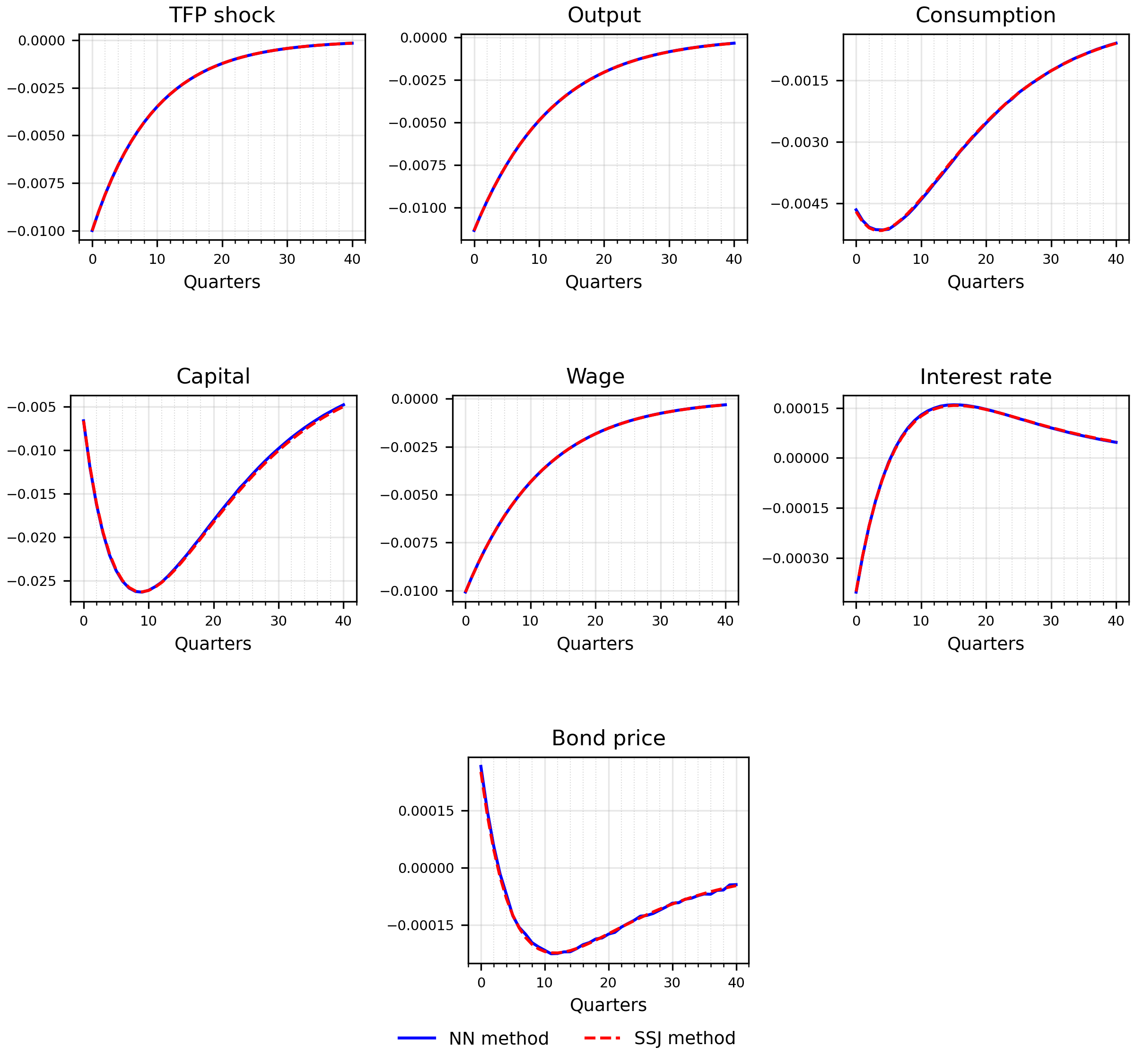
Finally, the figure below shows the equilibrium responses of selected aggregate variables to a negative TFP shock. The responses are expressed as deviations from the stochastic steady state. To prevent idiosyncratic household shocks from affecting the reported responses, the impulse response functions are averaged across 200 simulated economies that share the same idiosyncratic shocks with their unshocked counterparts. The dashed lines are the linearized SSJ responses from the deterministic steady state.
The impulse responses show that the trained neural networks generate stable and economically meaningful aggregate dynamics in the two-asset environment. Thus, the exercise evaluates not only the accuracy of the household first-order conditions but also the ability of the method to accurately approximate the general equilibrium dynamics of the two-asset model.