Extension 6: Observed variables
We now choose which model variables enter the data.
Model
This extension concerns the observation equation for the particle filter. The economy and calibration are those of Extension 5. So far, we have implicitly included all five variables determined in the model, \(\hat X_t\), \(\hat\Pi_t\), \(\hat I_t\), \(\hat R_t^*\), and \(\widehat{mp}_t\). These data are observed with some measurement error. The measurement equation is then given as
\[ \begin{bmatrix}\text{Output gap}\\\text{Inflation}\\\text{Interest rate}\\\text{Natural rate of interest}\\\text{Monetary policy shock}\end{bmatrix} =\begin{bmatrix}\hat X_t\\\hat\Pi_t\\\hat I_t\\\hat R_t^*\\\widehat{mp}_t\end{bmatrix}+u_t, \]
where the measurement error follows a Gaussian distribution \(u_t\sim N(0,\Sigma_u)\). The errors are independent across series, and the variance of the measurement error for each time series is a fraction \(m_E\) of its own variance. We set \(m_E=0.1\).
In this extension, we are interested in only observing the output gap, inflation, and the interest rate. The measurement equation is then given as
\[ \begin{bmatrix}\text{Output gap}\\\text{Inflation}\\\text{Interest rate}\end{bmatrix} =\begin{bmatrix}\hat X_t\\\hat\Pi_t\\\hat I_t\end{bmatrix}+u_t. \]
Neural network solution
Formulation
The policy network is unchanged. The filter still tracks all three states, but it uses only the three observed variables to calculate the likelihood.
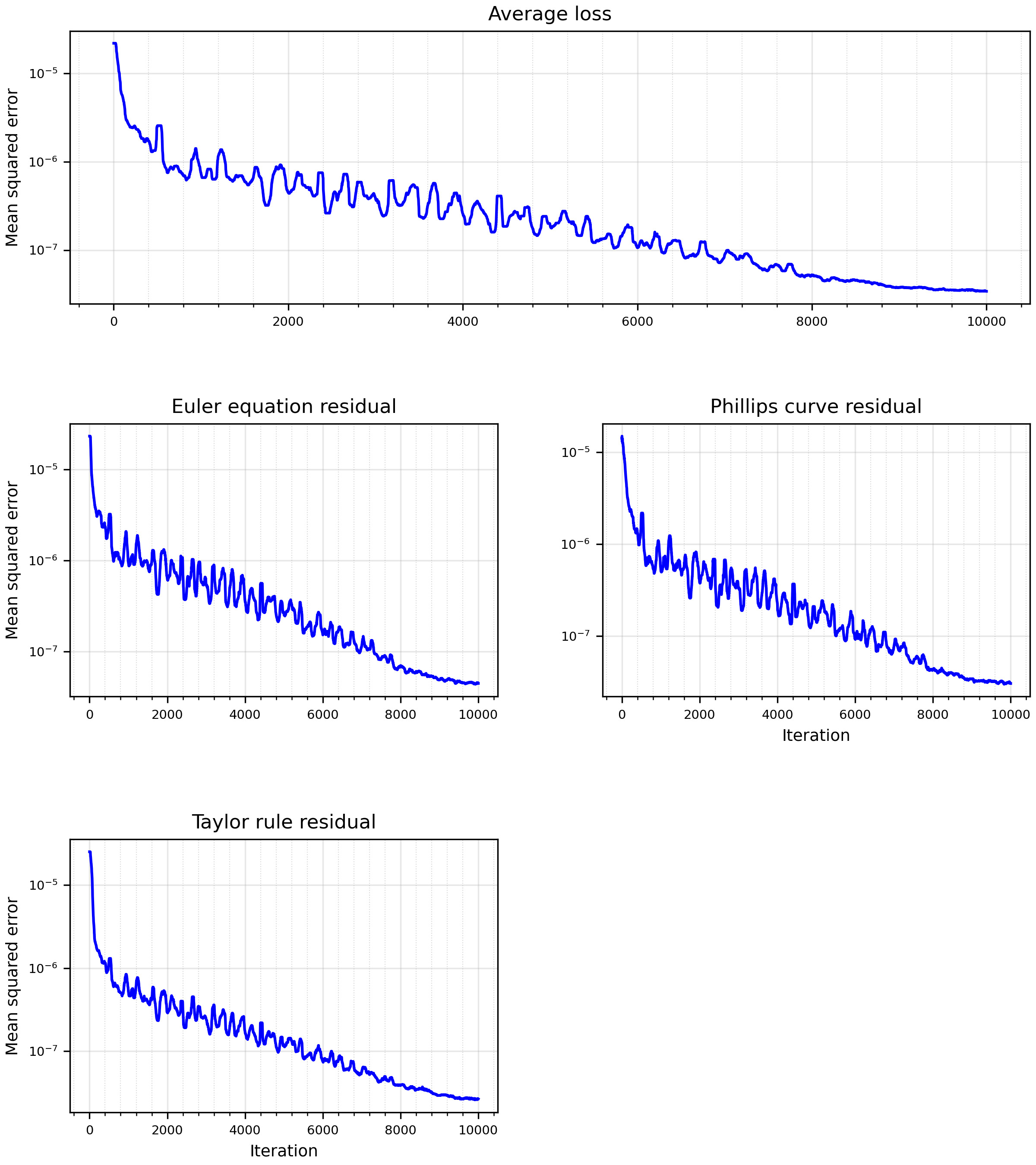
The loss is unchanged from Extension 1. It is the weighted mean of the squared residuals \(F_1\) (Euler equation), \(F_2\) (Phillips curve), and \(F_3\) (Taylor rule), with expectations approximated by Monte Carlo shock draws.
In the code
Select observations after evaluating policies
forecast advances the state and evaluates the policies, then observe selects the variables in OBSERVATION_NAMES, here the output gap, inflation, and the nominal rate. Both the simulation and the particle filter call this same method, so their observation definitions agree.
examples/rank/rank_extension_06.py
def observe(self, obs_raw):
    # New in Extension 6: observe only the three policy variables.
return {key: obs_raw[key] for key in self.OBSERVATION_NAMES}The notebook adds measurement noise after simulation and passes its covariance matrix to ParticleFilter. The natural rate and monetary shock remain in the model even though we no longer observe them.
Results
Solution
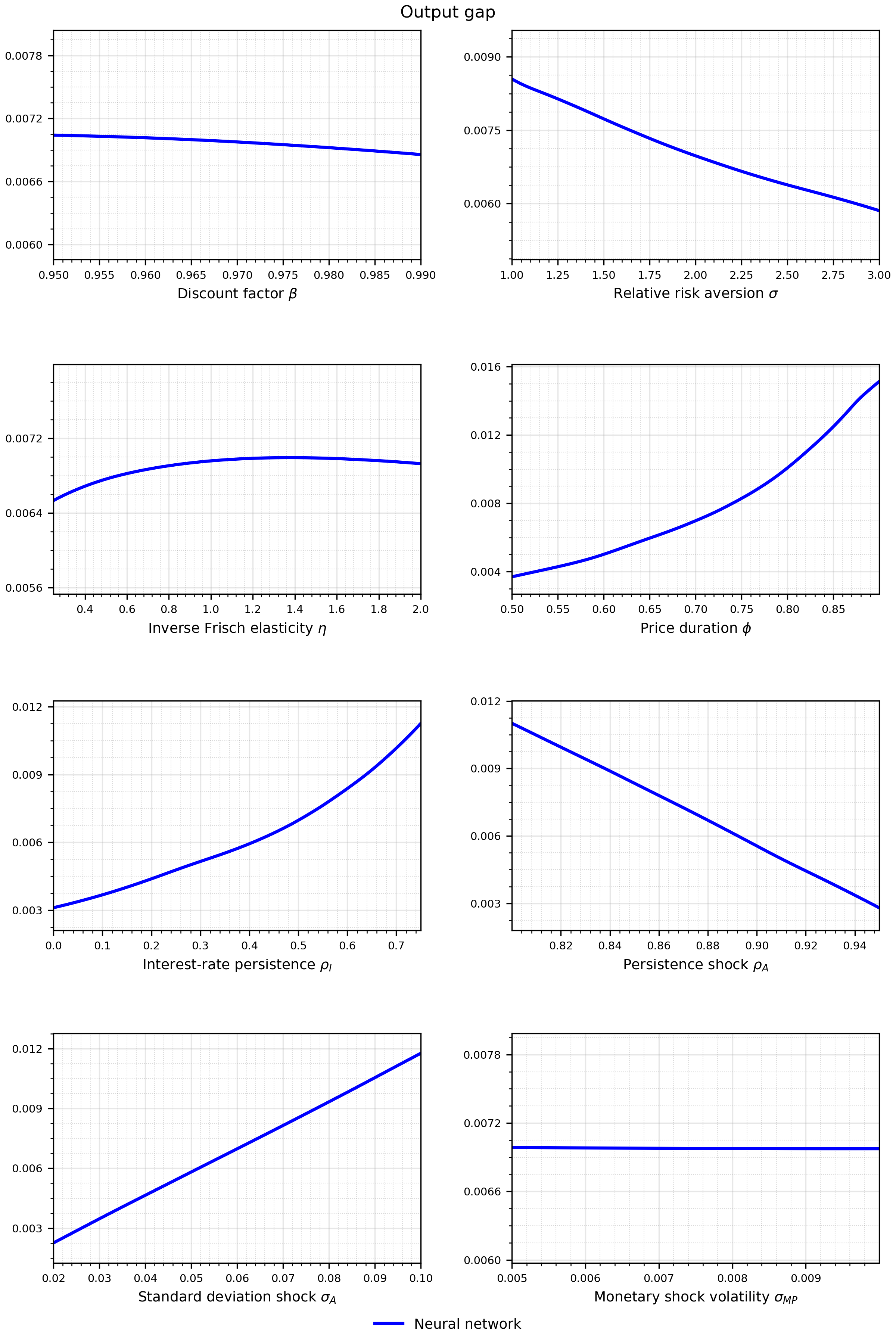
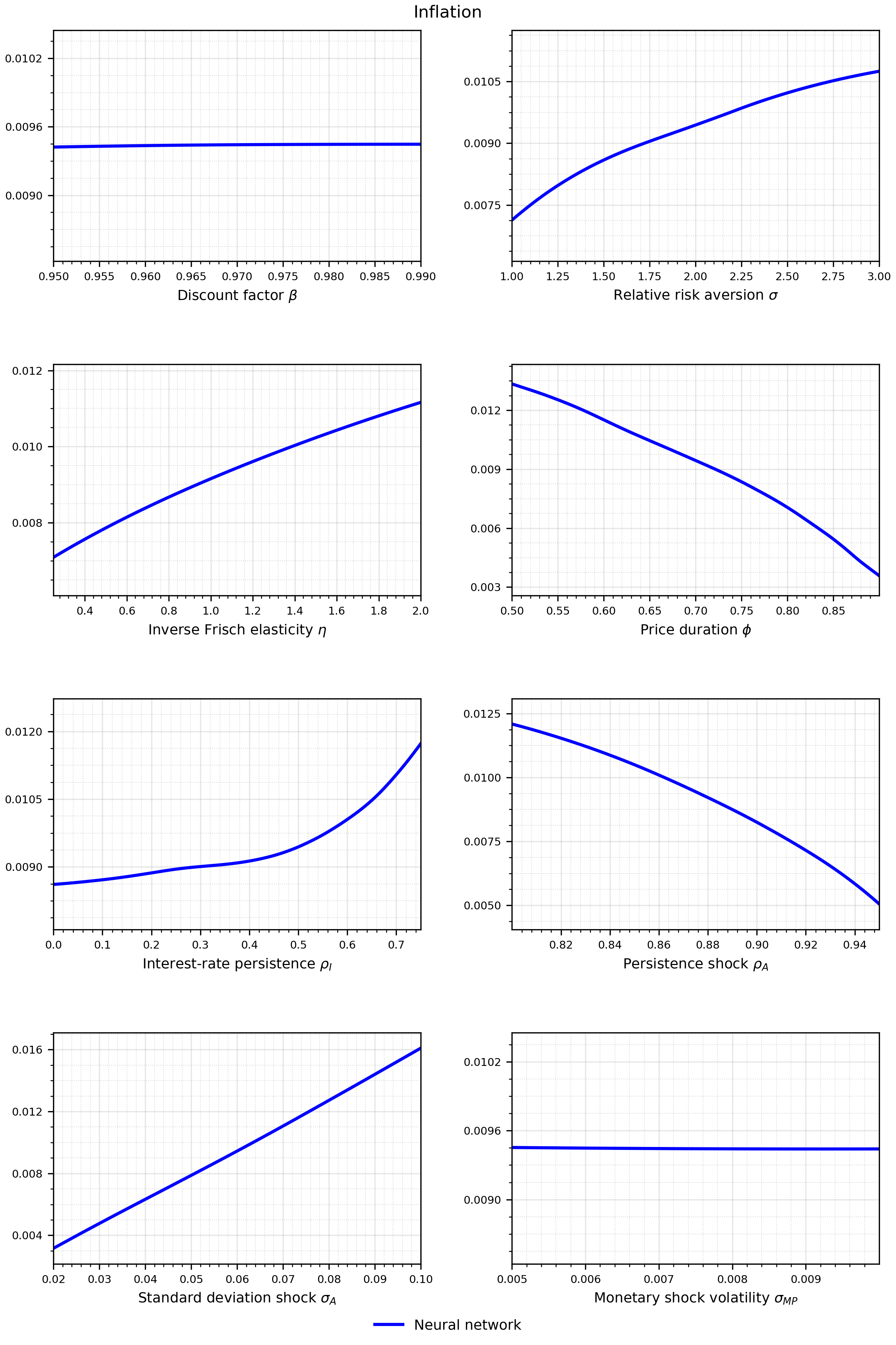
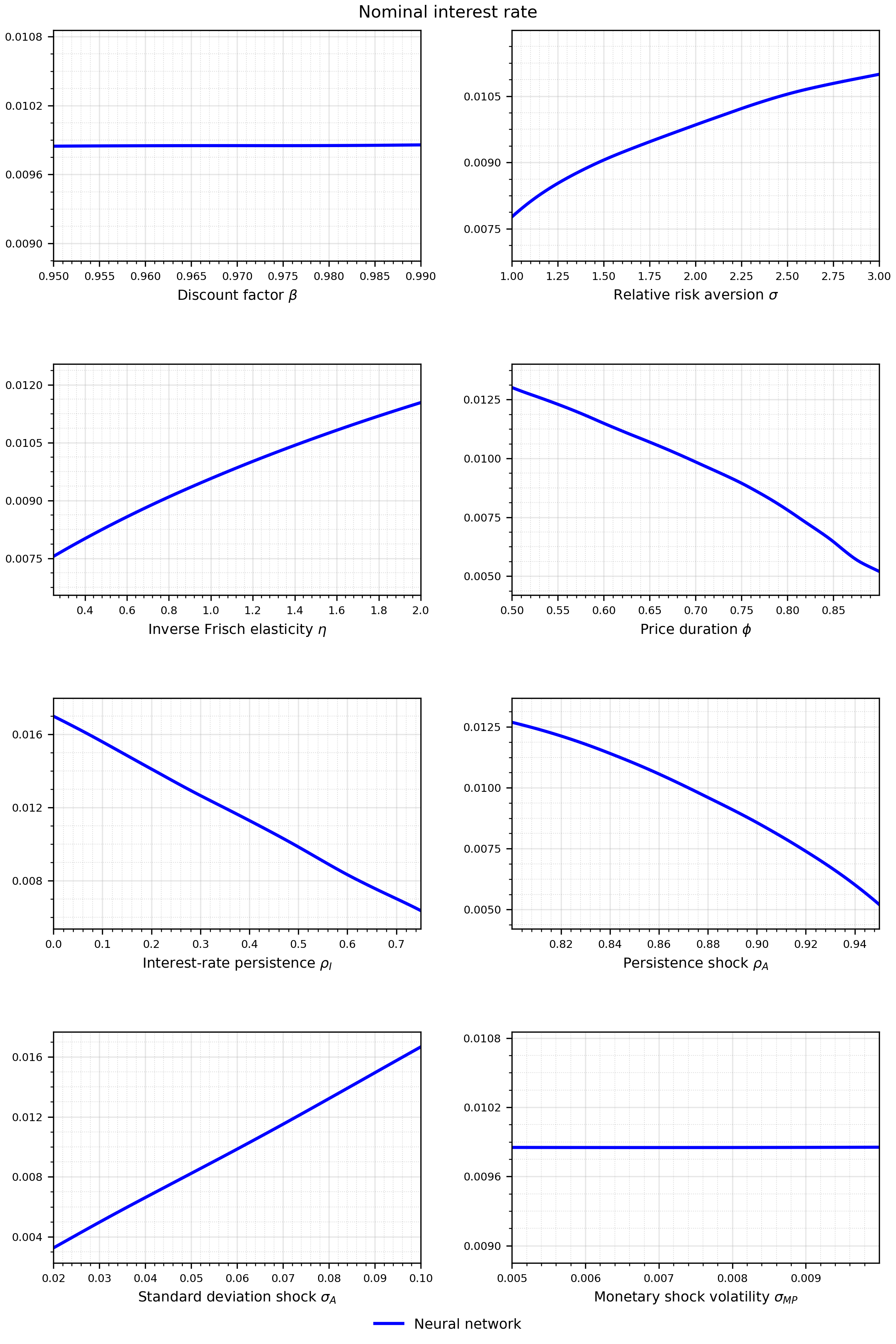
Likelihood