Heterogeneous households and monetary policy
Households differ in productivity and wealth. Their saving decisions determine the asset distribution. We include this distribution in the state when solving for aggregate prices. We first solve the economy without aggregate risk, then introduce monetary-policy shocks.
The script coordinates separate model, analysis, and plotting files, as in the paper’s replication package. Its saved networks are the trained networks from that package, so the script reproduces the paper’s solution without retraining. Run it from the environment described in Setting up Python.
Model
Households
Household \(i\) chooses consumption \(C_t^i\), labor \(H_t^i\), and bonds \(B_t^i\) to maximize
\[E_0\sum_{t=0}^{\infty}\beta^t\left[ \frac{(C_t^i)^{1-\sigma}}{1-\sigma}-\chi\frac{(H_t^i)^{1+\eta}}{1+\eta}\right].\]
Its budget and borrowing constraint are
\[C_t^i+B_t^i=W_te^{s_t^i}H_t^i+ \frac{R_{t-1}}{\Pi_t}B_{t-1}^i+(Div_t-T_t)e^{s_t^i},\qquad B_t^i\geq\underline B=0.\]
Here \(R_t\) is the gross nominal interest rate and \(\Pi_t\) is gross inflation. Idiosyncratic log productivity has an AR(1) transition. In each simulated panel of households, we recenter the draws so that mean productivity is one,
\[\widetilde s_{t+1}^i=\rho_s s_t^i+\sigma_s\epsilon_{t+1}^{s,i},\qquad s_{t+1}^i=\widetilde s_{t+1}^i-\log\left(\frac1L\sum_{j=1}^L e^{\widetilde s_{t+1}^j}\right),\]
where \(L\) is the number of households in the panel.
The innovations \(\epsilon^{s,i}\) and \(\epsilon^{mp}\) are independent standard normals. The optimality conditions are
\[\chi(H_t^i)^\eta=(C_t^i)^{-\sigma}W_te^{s_t^i},\]
\[1=\beta R_t E_t\left[\left(\frac{C_t^i}{C_{t+1}^i}\right)^\sigma \frac{1}{\Pi_{t+1}}\right]+\mu_t^i,\qquad \mu_t^i\geq0,\quad\mu_t^i(B_t^i-\underline B)=0.\]
Firms, policy, and markets
Output equals effective labor, \(Y_t=N_t=\int e^{s_t^i}H_t^i\,di\). With unit productivity, real marginal cost equals the wage, \(\Psi_t=W_t\). Rotemberg price adjustment gives
\[\varphi\log\Pi_t=(1-\epsilon)+\epsilon \Psi_t+ \varphi E_t\left[\frac{\Pi_{t+1}}{R_t}\log\Pi_{t+1}\frac{Y_{t+1}}{Y_t}\right].\]
Profits are \(Div_t=Y_t-W_tN_t-\tfrac12\varphi(\log\Pi_t)^2Y_t\). The nominal interest rate follows
\[R_t=R_{DSS}+\theta_\Pi(\Pi_t-1)+mp_t,\]
\[mp_{t+1}=\rho_{mp}mp_t+\sigma_{mp}\epsilon_{t+1}^{mp}.\]
Taxes \(T_t=(R_{t-1}/\Pi_t-1)D\) service fixed public debt \(D\). Market clearing requires
\[\int B_t^i\,di=D,\qquad \int C_t^i\,di+\tfrac12\varphi(\log\Pi_t)^2Y_t=Y_t.\]
Calibration
The household parameters come from the SSJ steady-state solve, which targets a steady-state nominal rate of 1.005. The code uses them at full precision. The monetary-shock persistence \(\rho_{mp}\) varies over \([0.5, 0.7]\) during training and is evaluated at 0.6.
| Household parameters | Value | Aggregate parameters | Value |
|---|---|---|---|
| Discount factor \(\beta\) | 0.982244 | Demand elasticity \(\epsilon\) | 6 |
| Risk aversion \(\sigma\) | 2 | Price adjustment \(\varphi\) | 60 |
| Labor curvature \(\eta\) | 2 | Inflation response \(\theta_\Pi\) | 1.5 |
| Labor disutility \(\chi\) | 0.786433 | Public debt \(D\) | 5.6 |
| Productivity persistence \(\rho_s\) | 0.966 | Monetary persistence \(\rho_{mp}\) | 0.6, trained over \([0.5, 0.7]\) |
| Productivity shock SD \(\sigma_s\) | 0.129271 | Monetary shock SD \(\sigma_{mp}\) | 0.0025 |
Neural network solution
Formulation
Each household’s state is \((B_{t-1}^i,s_t^i)\). The aggregate state contains the joint household distribution, the lagged nominal interest rate, and the current monetary shock. We represent the distribution with 100 households sorted by assets. A separate panel of \(L=100\) households evaluates individual optimality conditions. The estimated and calibrated parameter sets are
\[\tilde\Theta=\{\rho_{mp}\},\qquad \bar\Theta=\{\beta,\sigma,\eta,\chi,\rho_s,\sigma_s,\epsilon,\varphi,\theta_\Pi,D,\sigma_{mp}\},\]
so every network takes \(\rho_{mp}\) as an input.
The solution has two stages.
- Deterministic steady state (DSS). Idiosyncratic risk remains active while aggregate risk is absent. One network predicts household labor and another predicts \((R_{DSS},Y_{DSS})\). Inflation is one and the wage is \((\epsilon-1)/\epsilon\).
- Stochastic economy. Initialize the household network with the DSS weights. Train it together with an aggregate network that returns \((\Pi_t,W_t)\), and keep the DSS network fixed.
Each network normalizes each input variable, projects it to 128 values, and adds these projections, then applies four hidden layers of 128 CELU units and a linear output layer. There is no activation after the initial projections. Once labor is predicted, consumption follows from labor optimality and bond choices follow from the budget constraint,
\[C_t^i=\left(\frac{W_te^{s_t^i}}{\chi(H_t^i)^\eta}\right)^{1/\sigma},\qquad B_t^i=W_te^{s_t^i}H_t^i+\frac{R_{t-1}}{\Pi_t}B_{t-1}^i+(Div_t-T_t)e^{s_t^i}-C_t^i.\]
Residuals and loss
The Fischer–Burmeister function \(\Psi^{FB}(a,b)=a+b-\sqrt{a^2+b^2}\) encodes complementarity. Let \(\bar\lambda_t^i=\beta R_tE_t[(C_t^i/C_{t+1}^i)^\sigma/\Pi_{t+1}]\). The implementation adds a numerical upper asset bound \(\overline B=125\) and uses
\[F^{1,i}_t=\begin{cases} \Psi^{FB}(B_t^i-\underline B,1-\bar\lambda_t^i), & B_t^i<0.8\overline B,\\ \Psi^{FB}(\overline B-B_t^i,\bar\lambda_t^i-1), & B_t^i\geq0.8\overline B. \end{cases}\]
The second branch switches to the upper-bound complementarity condition. After training, check that this numerical bound does not affect the solution.
Five aggregate residuals follow, in the same order in both stages. \(F^2\) is output consistency \(Y_t-Y_{DSS}\) in the DSS stage and the Phillips curve in the stochastic stage. \(F^3=D-\langle B_t\rangle\) and \(F^4=Y_t-\langle C_t\rangle-\tfrac12\varphi(\log\Pi_t)^2Y_t\) are bond and goods market clearing, where angle brackets denote means over the distribution panel. \(F^5\) and \(F^6\) are the same two conditions next period, one for each of the \(M\) shock draws.
Each aggregate residual is divided by its scale before squaring. The Phillips curve is divided by \(1-\epsilon\), output and goods clearing by output, and bond clearing by \(D\). For a batch of \(N_{batch}\) economies, the loss is
\[ \mathcal L=\frac1{N_{batch}}\sum_{b=1}^{N_{batch}}\left[ \alpha_1\frac1L\sum_{i=1}^L(F^{1,i,b})^2+\sum_{j=2}^{4}\alpha_j(F^{j,b})^2 +\frac1M\sum_{m=1}^M\left(\alpha_5(F^{5,b,m})^2+\alpha_6(F^{6,b,m})^2\right)\right], \]
with every weight \(\alpha_j\) equal to one.
Training
Each iteration takes 10 internal updates on a batch of \(N_{batch}=50\) economies. Each update draws \(M=100\) next-period shocks as antithetic pairs to approximate the expectations. The shocks that simulate the panel forward are not paired. Every 10 iterations, before the panel advances, \(\rho_{mp}\) is redrawn for each economy and the panel advances 5 periods. After the updates, the panel advances \(T^{sim}=5\) periods. In the stochastic stage, if any household’s bonds leave \([\underline B-50,\overline B+50]\), the panel restarts from the steady state.
Each stage runs 20,000 iterations with AdamW, weight decay 0.01, and gradient-norm clipping at 1. The learning rate warms up from \(10^{-5}\) to \(10^{-4}\) over the first 2,000 iterations, then follows cosine annealing to \(10^{-8}\). Idiosyncratic shock standard deviations rise from 10% to 100% of their target over the first 1,000 iterations. In the stochastic stage, monetary shocks start at 10% and rise to full size between iterations 1,000 and 2,000.
In the code
Set the parameters and shocks
ranges lists the one parameter that varies during training. The aggregate productivity input z is retained from the replication package with zero shock variance. Rn_ss supplies the reference rate used to initialize the simulated panels. The DSS network learns its own rate.
examples/hankmp/hankmp.py
parameters = {
    # Households, from the SSJ steady-state solve.
    "beta": 0.9822435537836073,
    "gamma": 2.0,
    "eta": 2.0,
    "chi": 0.7864334221642553,
    "rho_s": 0.966,
    "sigma_s": 0.12927103310486848,
    "B": 5.6,
    "phipi": 1.5,
    # Borrowing limit and numerical upper asset bound.
    "b_min": -0.0,
    "b_max": 125.0,
    # Reference nominal rate for initialization. The DSS network learns R_DSS.
    "Rn_ss": 1.005,
    # Dormant TFP process.
    "rho_z": 0.0,
    "sigma_z": 0.0,
    # Monetary-policy shock.
    "rho_mps": 0.6,
    "sigma_mps": 0.0025,
    # Firms.
    "varphi": 60.0,
    "theta": 6.0,
}
ranges = {"rho_mps": torch.distributions.Uniform(0.5, 0.7)}  # Varies during training.
shocks_ind = {"s": torch.distributions.Normal(0.0, 1.0)}
shocks_agg = {
    "z": torch.distributions.Normal(0.0, 1.0),
    "mps": torch.distributions.Normal(0.0, 1.0),
}The code names map to the symbols above as follows.
| Code | Symbol | Meaning |
|---|---|---|
n |
\(H_t^i\) | labor |
b, b_min, b_max |
\(B_t^i\), \(\underline B\), \(\overline B\) | bonds and their bounds |
s |
\(s_t^i\) | log productivity |
gamma |
\(\sigma\) | risk aversion |
theta |
\(\epsilon\) | demand elasticity |
varphi |
\(\varphi\) | price-adjustment cost |
phipi |
\(\theta_\Pi\) | Taylor-rule inflation response |
B |
\(D\) | public debt |
tau |
tax per unit of \(e^{s_t^i}\) | |
Psi |
\(\Psi_t\) | real marginal cost |
NE |
\(N_t\) | productivity-weighted labor, equal to output \(Y_t\) |
Rn, Rn_lag, Rn_dss |
\(R_t\), \(R_{t-1}\), \(R_{DSS}\) | gross nominal rates |
mps, rho_mps, sigma_mps |
\(mp_t\), \(\rho_{mp}\), \(\sigma_{mp}\) | monetary shock |
lambda_comp |
\(\bar\lambda_t^i\) | expected Euler term |
Efp |
expected Phillips-curve term | |
res_fb, res_nkpc or res_y |
\(F^1\), \(F^2\) | household residual, Phillips curve (output consistency in the DSS) |
res_bond, res_product |
\(F^3\), \(F^4\) | market clearing today |
res_bond_next, res_product_next |
\(F^5\), \(F^6\) | market clearing next period |
_ind, _dist suffixes |
the \(L\)-household panel and the distribution panel |
Evaluate and transform policies
hh_policy sorts the distribution by assets, assembles the inputs, evaluates the household network, and transforms its output into labor. Consumption and bond holdings are then derived using the equations above. agg_policy follows the same sequence for the aggregate network, with separate columns for inflation and the wage. The output bounds help keep trial policies economically meaningful.
examples/hankmp/hankmp_model.py
def hh_policy(self, state_ind, state_dist, state_agg, par, mc=None):
    """Household labor n in (0.01, 2.0) from the full-model hh network (distribution sorted by assets)."""
    state_dist = self._permute_dist(state_dist.sort("b", dim=-2), mc)
    par = self._prepare_par_input(par, mc)
    out = self.hh_network(state_ind=state_ind, state_dist=state_dist, state_agg=state_agg, par=par)
    n_low, n_high = 0.01, 2.0
    return n_low + torch.sigmoid(out[..., 0:1]) * (n_high - n_low)

def agg_policy(self, state_dist, state_agg, par, mc=None):
    """Aggregate policies from the agg network: inflation Pi in (0.9, 1.1) and wage W in (0.5, 1.5)."""
    state_dist = self._permute_dist(state_dist.sort("b", dim=-2), mc)
    par = self._prepare_par_input(par, mc)
    out = self.agg_network(state_dist=state_dist, state_agg=state_agg, par=par)
    Pi = 0.9 + torch.sigmoid(out[..., 0:1]) * (1.1 - 0.9)
    W = 0.5 + torch.sigmoid(out[..., 1:2]) * (1.5 - 0.5)
return Pi, WForm the equilibrium errors
The method below evaluates current policies and calculates consumption and bonds. It then advances the states with the shock draws in e, evaluates future policies, averages over the draws, and forms the six residuals. detach_next=True holds future-policy predictions fixed when differentiating today’s equation errors. Two switches appear in the code. known_dss is off in this example, so the learned \((R_{DSS},Y_{DSS})\) are used. adjusted_residuals is on, which applies the scaling described above.
examples/hankmp/hankmp_model.py
def residuals(self, e, mc, detach_next=True, scale_ind=1, scale_agg=1, adjusted_residuals=False):
    par = self.par_draw
    ss = self.ss
    state_ind, state_dist, state_agg = self.state_ind, self.state_dist, self.state_agg
    e_ind, e_dist, e_agg = e

    # Current period: policies -> aggregates -> household budgets
    if self.known_dss:
        Rn_dss, Y_dss = ss.Rn, ss.Y
    else:
        Rn_dss, Y_dss = self.dss_policy(par=par)
    n_ind = self.hh_policy(state_ind=state_ind, state_dist=state_dist, state_agg=state_agg, par=par)
    n_dist = self.hh_policy(state_ind=state_dist, state_dist=state_dist, state_agg=state_agg, par=par)
    Pi, W = self.agg_policy(state_dist=state_dist, state_agg=state_agg, par=par)

    Rn_lag = state_agg.Rn_lag
    NE = torch.mean(torch.exp(state_dist.s) * n_dist, dim=-2, keepdim=True)
    Y = torch.exp(state_agg.z) * NE
    T = self._bond_tax(par.B, Rn_lag, Pi)
    tau = T / torch.mean(torch.exp(state_dist.s), dim=-2, keepdim=True)
    Psi = W / torch.exp(state_agg.z)
    Rn = Rn_dss + par.phipi * (Pi - 1) + state_agg.mps   # Taylor rule (ELB stripped)

    c_ind = ((W * torch.exp(state_ind.s)) / (ss.chi * n_ind ** par.eta)) ** (1 / par.gamma)
    c_dist = ((W * torch.exp(state_dist.s)) / (ss.chi * n_dist ** par.eta)) ** (1 / par.gamma)
    div = Y - W * NE - 0.5 * par.varphi * torch.log(Pi) ** 2 * Y
    div_ind = div * torch.exp(state_ind.s)
    div_dist = div * torch.exp(state_dist.s)
    wealth_ind = W * torch.exp(state_ind.s) * n_ind + Rn_lag / Pi * state_ind.b + div_ind - tau * torch.exp(state_ind.s)
    wealth_dist = W * torch.exp(state_dist.s) * n_dist + Rn_lag / Pi * state_dist.b + div_dist - tau * torch.exp(state_dist.s)
    b_ind = wealth_ind - c_ind
    b_dist = wealth_dist - c_dist
    C = torch.mean(c_dist, dim=-2, keepdim=True)

    # Next period
    shape_ind = e_ind.s.shape
    shape_dist = e_dist.s.shape
    shape_agg = e_agg.z.shape

    s_ind_next = self._ar1_next(state_ind.s, e_ind.s, par, scale_ind)
    s_dist_next = self._ar1_next(state_dist.s, e_dist.s, par, scale_ind)
    z = (1 - par.rho_z) * ss.z + par.rho_z * state_agg.z + e_agg.z * par.sigma_z * scale_agg
    mps = par.rho_mps * state_agg.mps + e_agg.mps * par.sigma_mps * scale_agg

    state_ind_next = State({"b": b_ind.expand(shape_ind), "s": s_ind_next})
    state_dist_next = State({"b": b_dist.expand(shape_dist), "s": s_dist_next})
    state_agg_next = State({"z": z, "mps": mps, "Rn_lag": Rn.expand(shape_agg)})

    with torch.set_grad_enabled(not detach_next):
        n_ind_next = self.hh_policy(mc=mc, state_ind=state_ind_next, state_dist=state_dist_next, state_agg=state_agg_next, par=par)
        n_dist_next = self.hh_policy(mc=mc, state_ind=state_dist_next, state_dist=state_dist_next, state_agg=state_agg_next, par=par)
        Pi_next, W_next = self.agg_policy(mc=mc, state_dist=state_dist_next, state_agg=state_agg_next, par=par)

    NE_next = torch.mean(torch.exp(state_dist_next.s) * n_dist_next, dim=-2, keepdim=True)
    Y_next = torch.exp(state_agg_next.z) * NE_next
    T_next = self._bond_tax(par.B, state_agg_next.Rn_lag, Pi_next)
    tau_next = T_next / torch.mean(torch.exp(state_dist_next.s), dim=-2, keepdim=True)
    div_next = Y_next - W_next * NE_next - 0.5 * par.varphi * torch.log(Pi_next) ** 2 * Y_next
    div_dist_next = div_next * torch.exp(state_dist_next.s)
    wealth_dist_next = W_next * torch.exp(state_dist_next.s) * n_dist_next + Rn / Pi_next * state_dist_next.b + div_dist_next - tau_next * torch.exp(state_dist_next.s)
    c_ind_next = ((W_next * torch.exp(state_ind_next.s)) / (ss.chi * n_ind_next ** par.eta)) ** (1 / par.gamma)
    c_dist_next = ((W_next * torch.exp(state_dist_next.s)) / (ss.chi * n_dist_next ** par.eta)) ** (1 / par.gamma)
    b_dist_next = wealth_dist_next - c_dist_next
    C_next = torch.mean(c_dist_next, dim=-2, keepdim=True)

    q = par.beta * (c_ind_next / c_ind) ** (-par.gamma)
    Efp = torch.mean((Pi_next / Rn) * torch.log(Pi_next) * (Y_next / Y), dim=0)
    lambda_comp = torch.mean(q * Rn / Pi_next, dim=0)

    # Equilibrium residuals (Euler/FB, NKPC, bond clearing, goods clearing)
    res_fb = torch.where(
        b_ind < 0.8 * par.b_max,
        fisher_burmeister(b_ind - par.b_min, 1 - lambda_comp),
        fisher_burmeister(par.b_max - b_ind, lambda_comp - 1),  # corrected sign (upper bound)
    )
    res_nkpc = par.varphi * torch.log(Pi) - ((1 - par.theta) + par.theta * Psi + par.varphi * Efp)
    res_bond = par.B - torch.mean(b_dist, dim=-2, keepdim=True)
    res_bond_next = par.B - torch.mean(b_dist_next, dim=-2, keepdim=True)
    res_product = Y - (C + 0.5 * par.varphi * torch.log(Pi) ** 2 * Y)
    res_product_next = Y_next - (C_next + 0.5 * par.varphi * torch.log(Pi_next) ** 2 * Y_next)

    if adjusted_residuals:
        return [res_fb, res_nkpc / (1 - par.theta), res_bond / par.B, res_product / Y, res_bond_next / par.B, res_product_next / Y_next]
return [res_fb, res_nkpc, res_bond, res_product, res_bond_next, res_product_next]The DSS version has the same structure. Inflation and the wage are fixed at their steady-state values, the rate is the learned \(R_{DSS}\), and the second residual is output consistency instead of the Phillips curve.
examples/hankmp/hankmp_model.py
def dss_residuals(self, e, mc, detach_next=True, scale_ind=1, scale_agg=0, adjusted_residuals=False):
    par = self.par_draw
    ss = self.ss
    state_ind, state_dist, state_agg = self.state_ind, self.state_dist, self.state_agg
    e_ind, e_dist, e_agg = e

    # Current period: policies -> aggregates -> household budgets
    n_ind = self.dss_hh_policy(state_ind=state_ind, state_dist=state_dist, state_agg=state_agg, par=par)
    n_dist = self.dss_hh_policy(state_ind=state_dist, state_dist=state_dist, state_agg=state_agg, par=par)
    if self.known_dss:
        Rn_dss, Y_dss = ss.Rn, ss.Y
    else:
        Rn_dss, Y_dss = self.dss_policy(par=par)

    Rn_lag = Rn_dss          # gross nominal rate on bonds (DSS: notional = SS level)
    Rn = Rn_dss              # realized gross nominal rate (DSS: no inflation gap, no mps)
    Pi = ss.Pi
    W = ss.W
    NE = torch.mean(torch.exp(state_dist.s) * n_dist, dim=-2, keepdim=True)
    Y = torch.exp(ss.z) * NE
    T = self._bond_tax(par.B, Rn_lag, Pi)
    tau = T / torch.mean(torch.exp(state_dist.s), dim=-2, keepdim=True)

    c_ind = ((W * torch.exp(state_ind.s)) / (ss.chi * n_ind ** par.eta)) ** (1 / par.gamma)
    c_dist = ((W * torch.exp(state_dist.s)) / (ss.chi * n_dist ** par.eta)) ** (1 / par.gamma)
    div = Y - W * NE - 0.5 * par.varphi * torch.log(Pi) ** 2 * Y
    div_ind = div * torch.exp(state_ind.s)
    div_dist = div * torch.exp(state_dist.s)
    wealth_ind = W * torch.exp(state_ind.s) * n_ind + Rn_lag / Pi * state_ind.b + div_ind - tau * torch.exp(state_ind.s)
    wealth_dist = W * torch.exp(state_dist.s) * n_dist + Rn_lag / Pi * state_dist.b + div_dist - tau * torch.exp(state_dist.s)
    b_ind = wealth_ind - c_ind
    b_dist = wealth_dist - c_dist
    C = torch.mean(c_dist, dim=-2, keepdim=True)

    # Next period
    shape_ind = e_ind.s.shape
    shape_dist = e_dist.s.shape
    shape_agg = e_agg.z.shape

    s_ind_next = self._ar1_next(state_ind.s, e_ind.s, par, scale_ind)
    s_dist_next = self._ar1_next(state_dist.s, e_dist.s, par, scale_ind)
    z = (1 - par.rho_z) * ss.z + par.rho_z * state_agg.z + e_agg.z * par.sigma_z * scale_agg
    mps = par.rho_mps * state_agg.mps + e_agg.mps * par.sigma_mps * scale_agg

    state_ind_next = State({"b": b_ind.expand(shape_ind), "s": s_ind_next})
    state_dist_next = State({"b": b_dist.expand(shape_dist), "s": s_dist_next})
    state_agg_next = State({"z": z, "mps": mps, "Rn_lag": Rn.expand(shape_agg)})

    with torch.set_grad_enabled(not detach_next):
        n_ind_next = self.dss_hh_policy(mc=mc, state_ind=state_ind_next, state_dist=state_dist_next, state_agg=state_agg_next, par=par)
        n_dist_next = self.dss_hh_policy(mc=mc, state_ind=state_dist_next, state_dist=state_dist_next, state_agg=state_agg_next, par=par)

    NE_next = torch.mean(torch.exp(state_dist_next.s) * n_dist_next, dim=-2, keepdim=True)
    Pi_next = ss.Pi
    W_next = ss.W
    Y_next = torch.exp(ss.z) * NE_next
    T_next = self._bond_tax(par.B, state_agg_next.Rn_lag, Pi_next)
    tau_next = T_next / torch.mean(torch.exp(state_dist_next.s), dim=-2, keepdim=True)
    div_next = Y_next - W_next * NE_next - 0.5 * par.varphi * torch.log(Pi_next) ** 2 * Y_next
    div_dist_next = div_next * torch.exp(state_dist_next.s)
    wealth_dist_next = W_next * torch.exp(state_dist_next.s) * n_dist_next + Rn / Pi_next * state_dist_next.b + div_dist_next - tau_next * torch.exp(state_dist_next.s)
    c_ind_next = ((W_next * torch.exp(state_ind_next.s)) / (ss.chi * n_ind_next ** par.eta)) ** (1 / par.gamma)
    c_dist_next = ((W_next * torch.exp(state_dist_next.s)) / (ss.chi * n_dist_next ** par.eta)) ** (1 / par.gamma)
    b_dist_next = wealth_dist_next - c_dist_next
    C_next = torch.mean(c_dist_next, dim=-2, keepdim=True)

    q = par.beta * (c_ind_next / c_ind) ** (-par.gamma)
    lambda_comp = torch.mean(q * Rn / Pi_next, dim=0)

    # Equilibrium residuals (Euler/FB, output, bond clearing, goods clearing)
    res_fb = torch.where(
        b_ind < 0.8 * par.b_max,
        fisher_burmeister(b_ind - par.b_min, 1 - lambda_comp),
        fisher_burmeister(par.b_max - b_ind, lambda_comp - 1),  # corrected sign (upper bound)
    )
    res_y = Y - Y_dss
    res_bond = par.B - torch.mean(b_dist, dim=-2, keepdim=True)
    res_bond_next = par.B - torch.mean(b_dist_next, dim=-2, keepdim=True)
    res_product = Y - (C + 0.5 * par.varphi * torch.log(Pi) ** 2 * Y)
    res_product_next = Y_next - (C_next + 0.5 * par.varphi * torch.log(Pi_next) ** 2 * Y_next)

    if adjusted_residuals:
        return [res_fb, res_y / Y, res_bond / par.B, res_product / Y, res_bond_next / par.B, res_product_next / Y_next]
return [res_fb, res_y, res_bond, res_product, res_bond_next, res_product_next]loss adds the weighted mean squared residuals into the training loss. It also returns each unweighted equation loss for the loss plots.
examples/hankmp/hankmp_model.py
def loss(self, residuals, criterion, names, weights=None):
    """Weighted sum of per-residual MSEs (the scalar to backprop) plus the unweighted per-residual components for logging."""
    if weights is None:
        weights = [1.0] * len(residuals)
    loss = [weights[i] * criterion(r, target=torch.zeros_like(r)) for i, r in enumerate(residuals)]
    with torch.no_grad():
        loss_components = {name: torch.mean(r ** 2) for name, r in zip(names, residuals)}
return sum(loss), loss_componentsTrain in two stages
The repository ships the trained networks from the replication package. Leave load_dss and load_full set to True to load them. Set load_full = False to retrain the stochastic model, and also set load_dss = False to solve the DSS again. The full-model checkpoint includes the DSS networks. Between the two stages, warm_start_full copies the DSS household weights into the stochastic model’s household network.
The computations are performed on an NVIDIA GeForce RTX 5090 GPU with 32 GB of memory. The computational time is around 43 minutes for the DSS and 46 minutes for the full equilibrium. The GPU memory usage is 0.6 GB. Training takes far longer on a CPU.
Both stages use the same training settings.
examples/hankmp/hankmp.py
# Both stages use the same settings. Aggregate residuals are divided by their scale.
config = TrainingConfig(
    iteration=20000,
    internal=10,
    steps=5,
    batch=50,
    mc=100,
    lr=1e-4,
    eta_min=1e-8,
    adjusted_residuals=True,
    device=DEVICE,
    seed=1234,
)
examples/hankmp/hankmp.py
dss_path = networks / "dss.pt"
full_path = networks / "full.pt"
train_full = not load_full or not full_path.exists()
train_dss = train_full and (not load_dss or not dss_path.exists())

if train_dss:
    print("Training the deterministic steady state...")
    model.train_dss_model(config)
    model.save(networks, name="dss")
    # A new DSS needs a new full model, so delete the saved one.
    full_path.unlink(missing_ok=True)
elif train_full:
    print("Loading the deterministic steady state.")
    model.load(dss_path)
examples/hankmp/hankmp.py
if train_full:
    print("Training the model with aggregate risk...")
    model.warm_start_full()
    model.train_model(config)
    model.save(networks, name="full")
else:
    print("Loading the model with aggregate risk.")
model.load(full_path)Results
The analysis uses the methods of the replication package with smaller samples, so it runs on a CPU in about 10 minutes. It compares with the SSJ reference shipped in examples/hankmp/outputs/reference. The results are saved and reused. Set load_analysis = False to recompute them.
Deterministic steady state
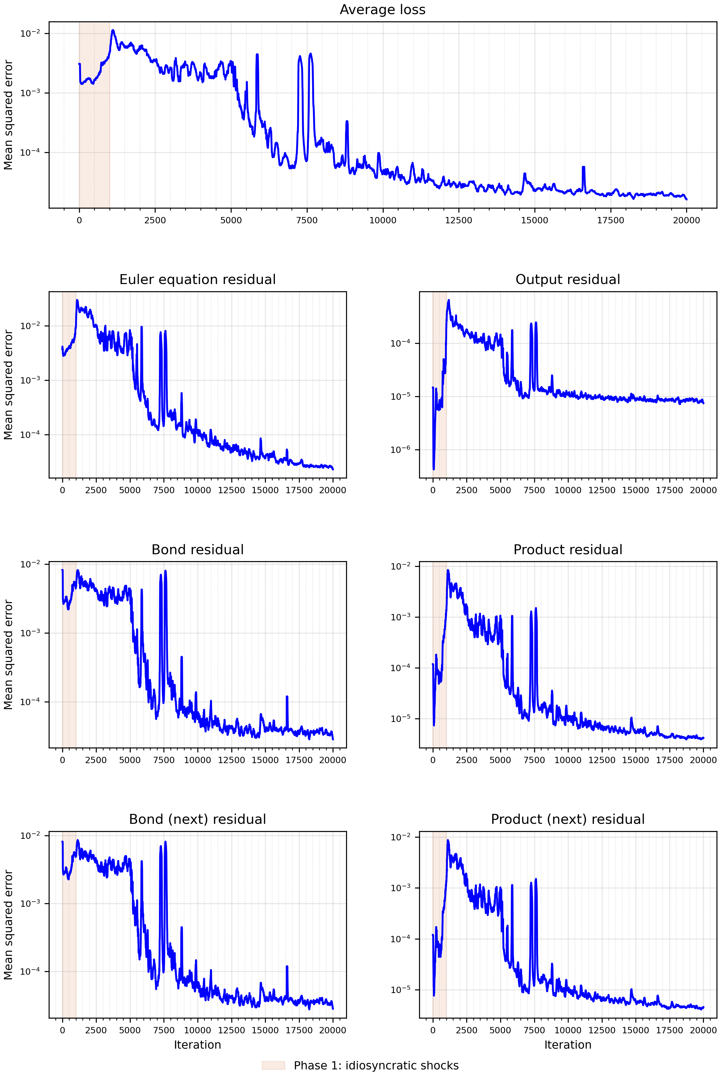
The top panel of the figure below displays the evolution of the average loss over the training. In the lower panels, we plot the in-training evolution of each equilibrium condition. To facilitate convergence during training, we gradually introduce idiosyncratic shocks by increasing their variance from a small value to their target levels over the course of the first 1,000 iterations. The red shaded area marks this stage. The training is successful, with clear convergence of the average loss. The breakdown of the loss into the individual residual errors confirms that the neural network learns all policy functions of interest effectively.
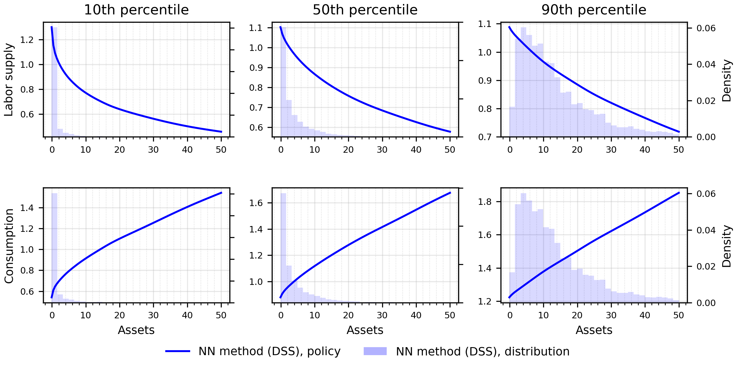
The next figure shows the bar graph of the asset distribution conditional on various levels of productivity (10th percentile, 50th percentile, and 90th percentile) along with the policy functions of labor supply and consumption. To be concise, we skip the values of the deterministic steady state here. The script calculates them.
Full equilibrium
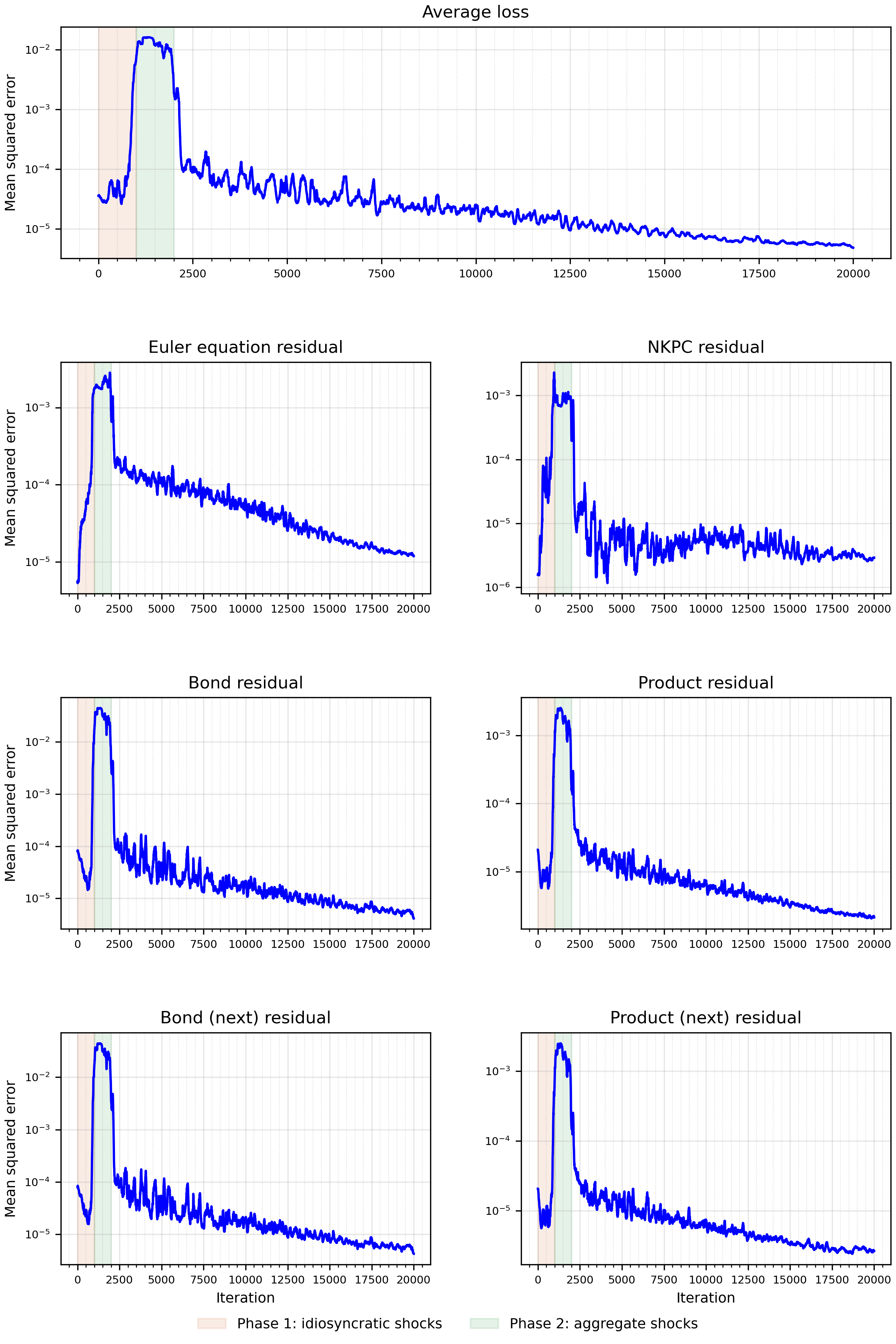
The top panel of the figure below displays the evolution of the average loss over the training for 20,000 iterations. In the other panels, we plot the in-training evolution of the Euler equation, the New Keynesian Phillips curve (NKPC), bond market clearing in the current as well as next period, and goods market clearing in the current as well as next period. As in the DSS, we gradually introduce idiosyncratic shocks over the first 1,000 iterations, marked by the red shaded area. Afterward, we introduce aggregate risk between iterations 1,000 and 2,000. The training is successful, with clear convergence of the average loss.
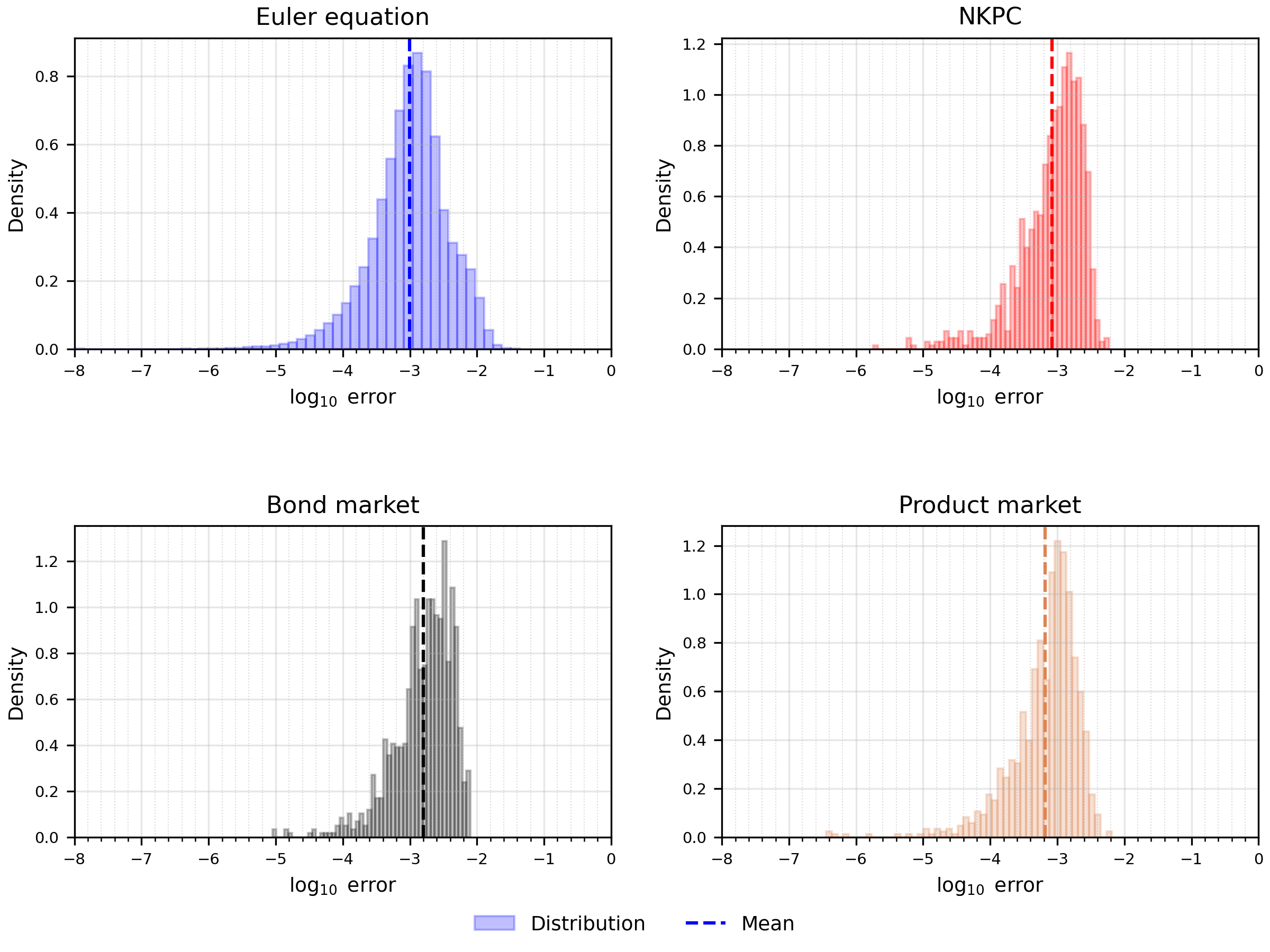
The next step is to calculate the approximation errors after the training of the neural networks has been completed. We use the same set of equilibrium conditions used during training, which are the Euler equation, the NKPC, bond market clearing, and goods market clearing. The absolute errors for these equations can be written as
\[ \begin{aligned} err_1 &= \left|\Psi^{FB}\left(1-\beta R_t\mathbb E_t\left[\left(\frac{C_t^i}{C_{t+1}^i}\right)^\sigma\frac{1}{\Pi_{t+1}}\right],B_t^i-\underline B\right)\right|,\\ err_2 &= \left|\frac{\varphi\log\Pi_t}{1-\epsilon}-\left(1+\frac{\epsilon}{1-\epsilon}\Psi_t+\frac{\varphi}{1-\epsilon}\mathbb E_t\left[\frac{\Pi_{t+1}}{R_t}\log\Pi_{t+1}\frac{Y_{t+1}}{Y_t}\right]\right)\right|,\\ err_3 &= \left|1-\frac{\frac1L\sum_{i=1}^L B_t^i}{D}\right|,\\ err_4 &= \left|1-\frac{\frac1L\sum_{i=1}^L C_t^i+\tfrac12\varphi(\log\Pi_t)^2Y_t}{Y_t}\right|, \end{aligned} \]
where \(err_1\) is for the Euler equation, \(err_2\) for the NKPC, \(err_3\) for bond market clearing, and \(err_4\) for goods market clearing. These are the scaled residuals used in training. We do not include bond and goods market clearing next period, as they are already covered by their current-period counterparts. We simulate 10 economies and calculate the approximation errors at 100 successive periods, drawing 1,000 shocks to evaluate expectations. The replication package uses 1,000 periods, for 10,000 observations in total. The residual errors are well contained. The symmetry and concentration of the distributions around small values further reinforce the reliability of the neural network solution, indicating that the approximation performs consistently well across a wide range of simulated states.
Comparison with the sequence-space Jacobian
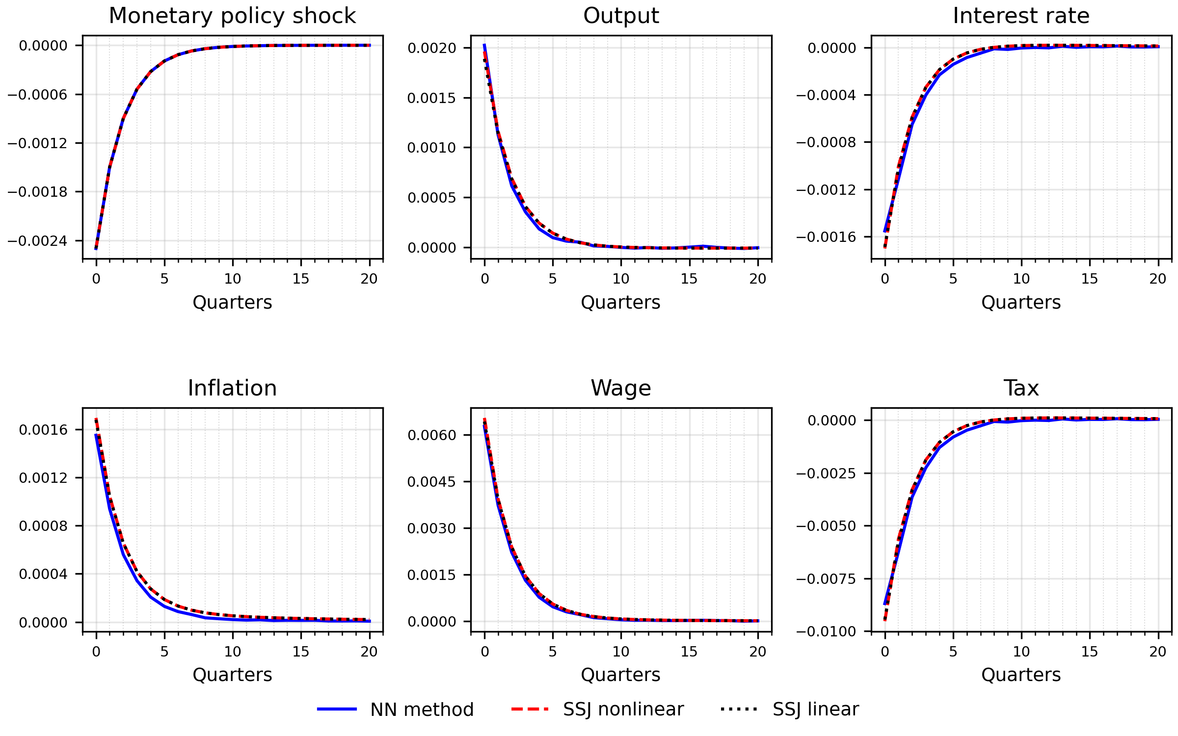
We now compare our neural network-based solution method to a conventional (linear) approach, specifically the sequence-space Jacobian (SSJ) approach of Auclert et al. (2021). For this comparison, we use the conventional linearized SSJ solution. The impulse responses also show the nonlinear SSJ solution.
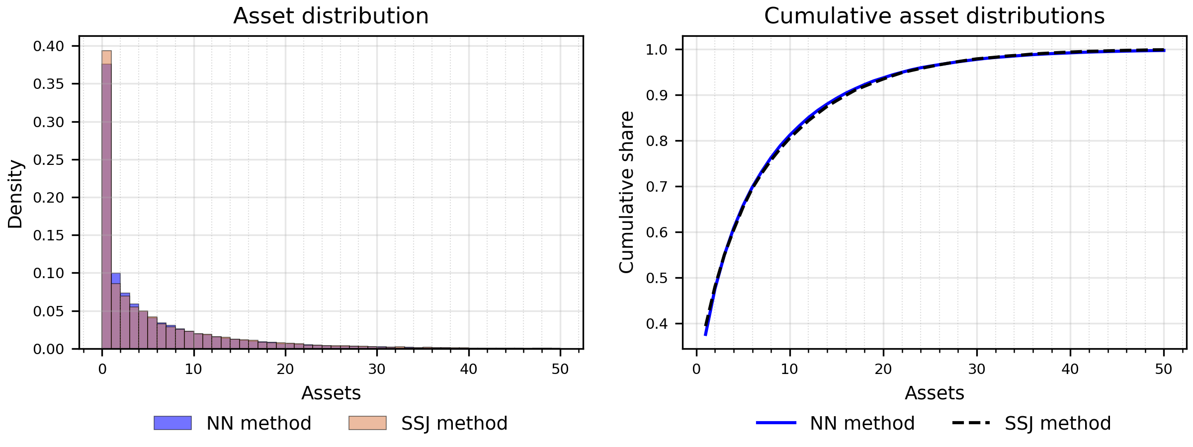
The figure below compares the asset distribution generated by our method and by the SSJ approach. For our method, we report the distribution averaged over economies simulated with aggregate shocks, which accounts for the presence of aggregate risk. In contrast, the linearized SSJ solution we use assumes away aggregate uncertainty in the steady state, so its distribution corresponds to the deterministic steady state. Despite this key difference, the two distributions are remarkably similar. Although minor deviations are visible in the tails, the overall shape and key moments align closely, suggesting that our method provides a highly accurate approximation. In the paper, we report the comparison using the deterministic steady state for both models. In this case, the resulting distributions are also remarkably similar, as expected.
Notably, these deviations cannot be attributed solely to inaccuracies in either our method or the SSJ approach. Instead, they stem from a fundamental difference in the economic environments captured by the two methods. Incorporating aggregate uncertainty, as our method does, leads poorer households to work more in response to increased precautionary motives, resulting in fewer households clustered at the bottom of the asset distribution, as reflected in the shorter blue bars in the lower asset bins. At the same time, this increased labor supply and precautionary saving among the poor depresses the equilibrium real interest rate, thereby reducing the incentive for wealthier households to save. As a result, rich households accumulate less wealth in equilibrium, leading to a thinner right tail in the asset distribution. This pattern is clearly illustrated by the crossing of the blue solid and black dashed lines in the right panel, which plots the cumulative asset distribution.
Even in this relatively stylized model, the differences between the asset distributions implied by the nonlinear (our method) and linearized (SSJ) solutions are already notable, despite being quite small. As we will show, these differences become even more pronounced if we increase aggregate risk.
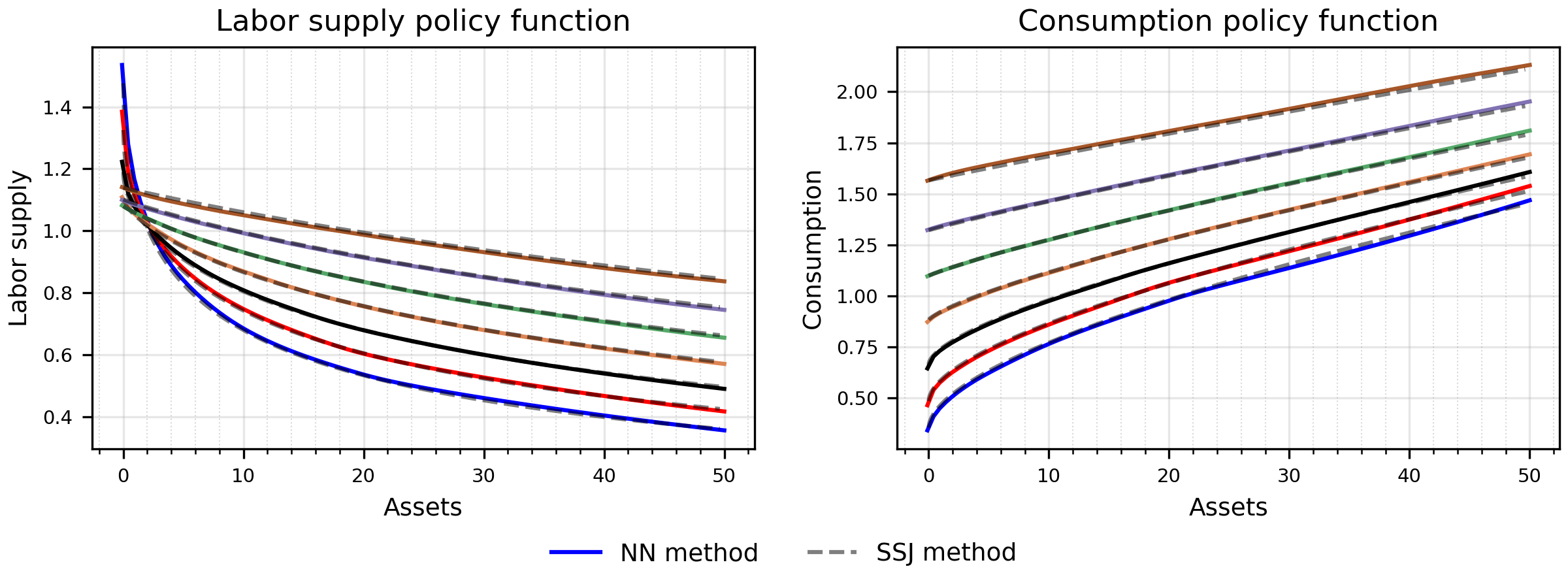
The next step is to compare the two sets of policy functions that determine agents’ labor supply and consumption decisions, as shown in the figure below. The solid lines depict the policy functions approximated using our method, while the dashed lines correspond to the approximation obtained using the SSJ method. Each color represents one of the seven idiosyncratic labor productivity levels considered in Auclert et al. (2021). The brown lines correspond to the most productive agents (top productivity bin), while the blue lines represent the least productive ones (bottom productivity bin).
These seven productivity levels are used solely for the purpose of comparing the results from our solution method with those from SSJ. Our solution method does not rely on discretizing the productivity space. Instead, we treat idiosyncratic labor productivity as the outcome of a continuous AR(1) process, as specified in the model. For the purpose of this comparison, we evaluate the policy functions at the values of the discretization in the code made available by Auclert and coauthors.
The upshot of the comparison is twofold. First, our method successfully replicates the policy functions approximated by the SSJ approach. Second, the main discrepancy arises in the behavior of the most productive agents with zero assets and of low productive agents with a large amount of assets. Both groups represent a tiny fraction of agents. Because so few agents follow such a path, the neural network has limited data to learn from, which results in a less accurate approximation of their behavior. Nonetheless, the inaccuracies in these cases are fairly limited, highlighting the strong extrapolative properties of neural networks.
Indeed, the effects of a monetary policy shock on the equilibrium dynamics of aggregate variables predicted by the two methods are quite similar, as the figure below shows.
Robustness
We now test how changing the number of agents and the number of draws for the Monte Carlo integration affects our results, and how the solution behaves for small and large shocks. These runs come from the replication package. Their networks are not shipped with this example, but their saved results in examples/hankmp/outputs/robustness are enough to draw the figures, and section 8 of the script redraws them. They use the full analysis sizes of the replication package, for example 2,000 economies for the asset distribution.
Number of agents
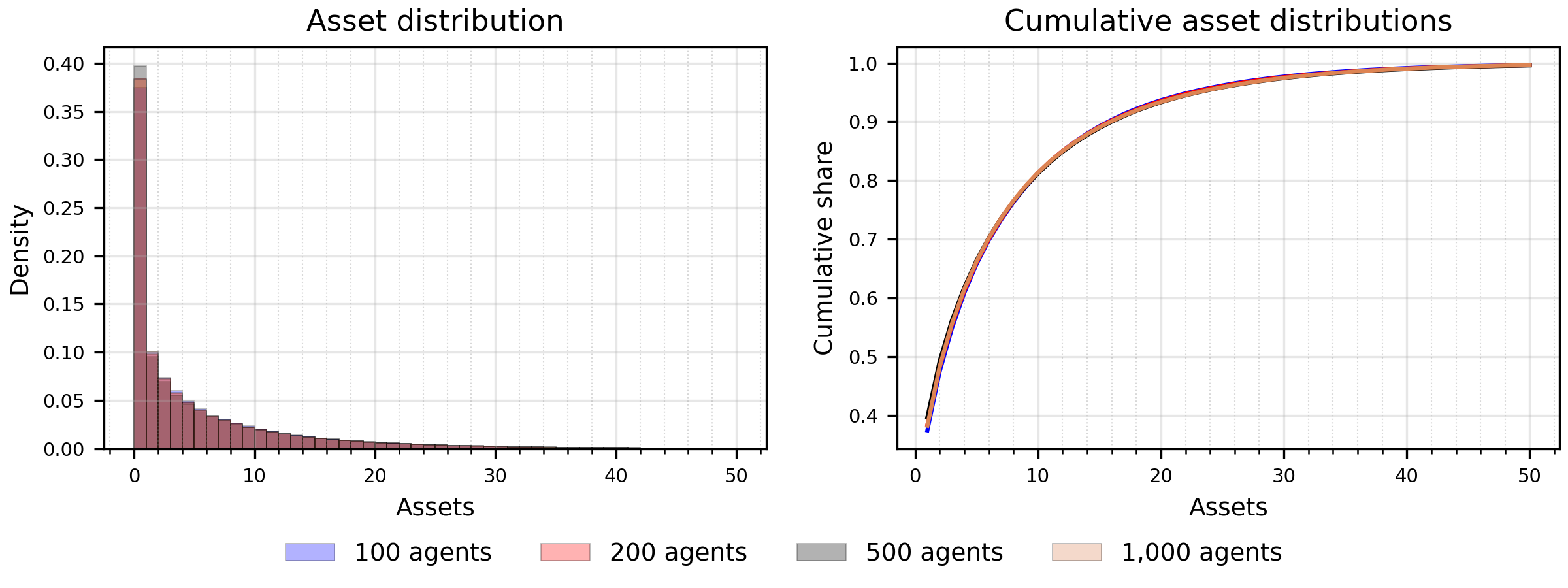
The figure below shows the distribution of asset holdings across different levels of discretization, with the left panel showing the histogram and the right panel the corresponding cumulative distribution function. We compare the results for \(L\)=100, 200, 500, and 1,000 agents. Each distribution is obtained by averaging across 2,000 simulated economies (batches). The two panels illustrate that the benefit of increasing the number of tracked agents to capture heterogeneity is minimal, since the asset distribution changes only slightly.
Even more striking is the comparison based on the policy functions for labor and consumption. The next figure shows the bar graph of the asset distribution conditional on various levels of productivity (10th percentile, 50th percentile, and 90th percentile) along with the policy functions of labor and consumption for 100 agents (solid line) and 1,000 (dashed line). The other individual policy function determines the agent’s asset demand, which is implied by the two individual policy functions and hence is not shown. The policy functions exhibit minimal change as the number of tracked agents increases from 100 to 1,000, supporting our claim that tracking more than 100 agents yields little additional benefit in approximating the asset distribution in this one-asset HANK model.
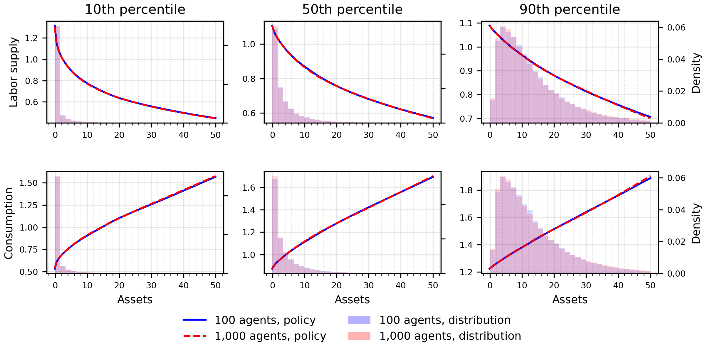
Nevertheless, computing time increases rapidly as the number of agents tracked \(L\) grows, as the table below shows. The runtime ranges from 1h31min for \(L=100\) to 6h12min for \(L=1,000\) on an NVIDIA RTX 5090 GPU with 32 GB of memory. Notably, even the version of the model with 1,000 agents required only 5.3 GB of memory (compared to just 0.6 GB for \(L=100\)). This reflects the memory-efficient design of our solution code, which makes it feasible to run the nonlinear one-asset HANK model on a desktop machine. For instance, solving the model with \(L=100\) took 30h38min on a recent MacBook with an Apple M4 Pro chip (14-core CPU and 20-core GPU), using the Metal framework for macOS devices. When run on the CPU, the same task took approximately twice as long.
| Number of agents | GPU computational time | GPU memory usage (GB) |
|---|---|---|
| \(L=100\) | 1h31min | 0.6 |
| \(L=200\) | 2h05min | 1.1 |
| \(L=500\) | 3h35min | 2.7 |
| \(L=1,000\) | 6h12min | 5.3 |
Number of Monte Carlo draws
We adopt a Monte Carlo approach to approximate expectations. In general, the accuracy of this approximation depends on using a sufficiently large number of Monte Carlo draws for next-period shock realizations. Here, we show that this number does not need to be large when using our neural network approach. In fact, a relatively modest number of draws is sufficient to achieve accurate approximations. The underlying reasons are similar to those that explain why only a limited number of agents need to be tracked in our framework.
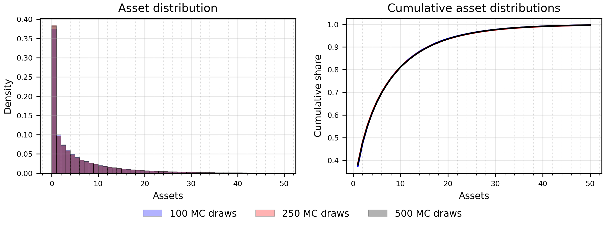
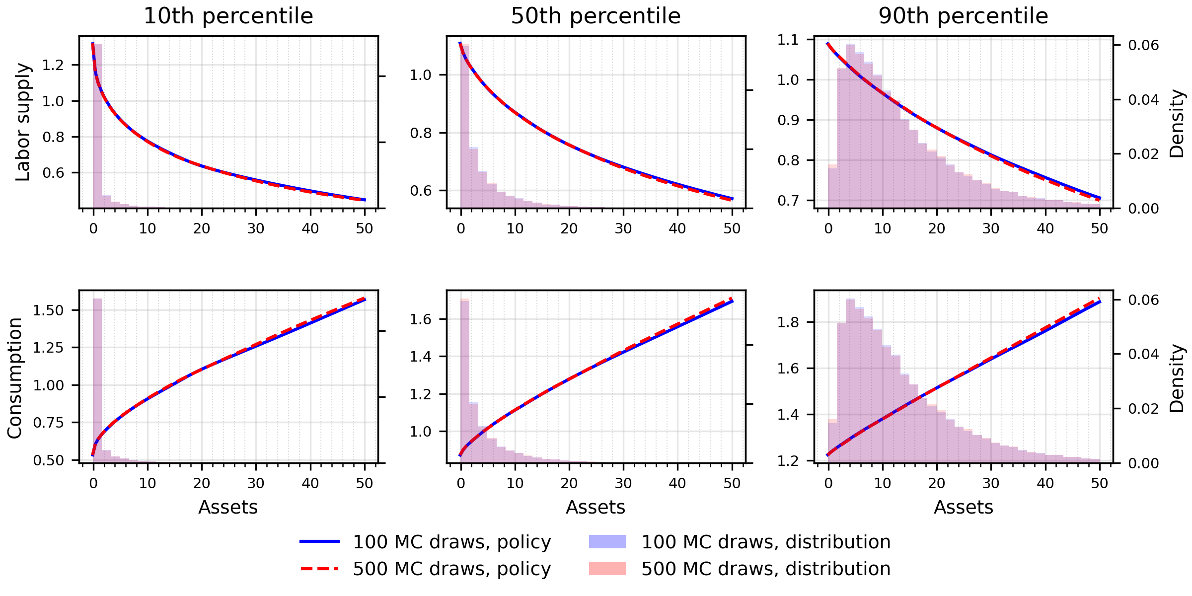
In the baseline case with 100 agents, we vary the number of Monte Carlo draws used to approximate next-period variables, testing with 100, 250, and 500 draws. The number of agents is fixed at \(L=100\) across these exercises. The results show that 100 Monte Carlo draws approximate the expectations very well here. One reason that they perform so well is that we take a new set of Monte Carlo draws during the training process for each iteration and batch, resulting in a very good approximation over the training process.
Size of shock volatility
The accuracy of the neural-network approximation can deteriorate when the volatility of aggregate shocks becomes extremely small. In this case, the variation induced by the aggregate shock may become difficult to distinguish from the numerical noise inherent in the training procedure.
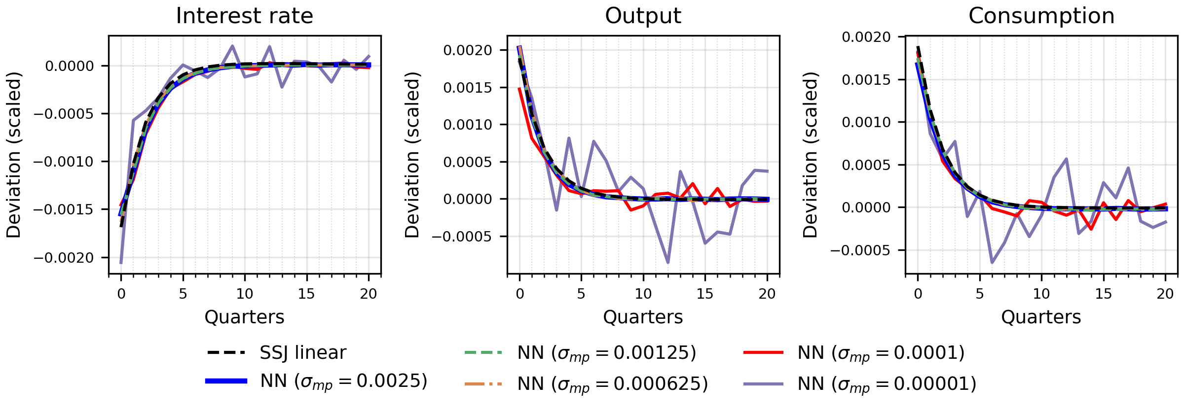
The figure below illustrates the case of very low volatility of the monetary policy shock. It shows how the accuracy of the neural-network solution changes as we progressively reduce the standard deviation \(\sigma_{mp}\) of the monetary policy innovation. In the benchmark specification, the standard deviation of this shock is 25 basis points. We then lower it to the values reported in the legend at the bottom of the figure. The neural-network solution remains stable when the standard deviation is reduced to 12.5 or 6.25 basis points. However, at implausibly low volatility levels, 1 basis point or less, the neural network begins to fail to capture the impulse responses to monetary policy shocks accurately.
The relevant issue is not the magnitude of the impulse responses themselves, which are rescaled to correspond to the same shock size, but the signal-to-noise ratio encountered during training. Our neural-network method relies on simulated data generated using a finite number of agents, Monte Carlo integration, and a finite sample of aggregate states. These ingredients inevitably introduce numerical noise into the training procedure. When aggregate volatility becomes sufficiently small, the variation generated by the aggregate shock becomes comparable to, or smaller than, this numerical noise. The neural network can then no longer reliably distinguish the aggregate signal from noise in the simulated environment.
The role of large aggregate uncertainty
The next step is to illustrate how, even in a HANK model with only one aggregate shock, an increase in aggregate risk leads to a substantial divergence between the solutions approximated with our code and the SSJ method. At higher levels of aggregate risk, precautionary saving behavior becomes more prominent, especially when intertwined with the model’s nonlinear features. To illustrate the effect, we scale the size of the monetary policy shock by a factor of ten, to \(\sigma_{mp}=0.025\). This run uses its own training recipe. It trains on raw residuals with weights of 10, a step learning-rate schedule, 25 updates per iteration, and a tighter normalization of the shock input.
With a larger standard deviation of monetary policy shocks, aggregate uncertainty increases and nonlinearities become more pronounced. This has substantial effects on the asset distribution, households’ policy functions, and the aggregate transmission of shocks. As shown in the figure below, the share of households near the borrowing limit is now significantly lower. As our method accounts for aggregate risk, we can now see a substantial difference compared to SSJ.
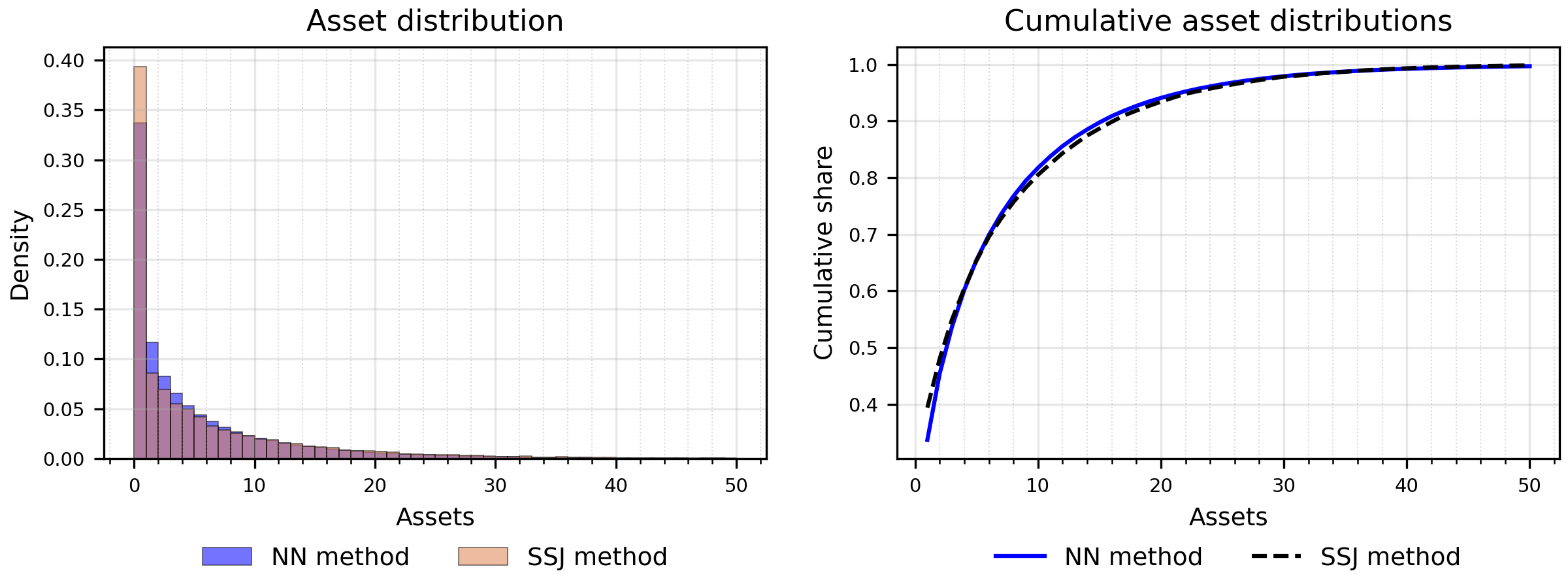
The underlying mechanism, which we already presented for the asset distribution in the baseline economy, is now amplified by the higher aggregate volatility. The precautionary savings motive leads households in low productivity states to work more and consume less, relative to a scenario with little or no aggregate risk, in order to accumulate buffer stocks of savings. Indeed, our NN solution method shows that there is now a much lower share of households near the borrowing limit because households have a larger precautionary motive due to larger aggregate risks. The linearized SSJ solution does not capture these effects on the equilibrium wealth distribution.
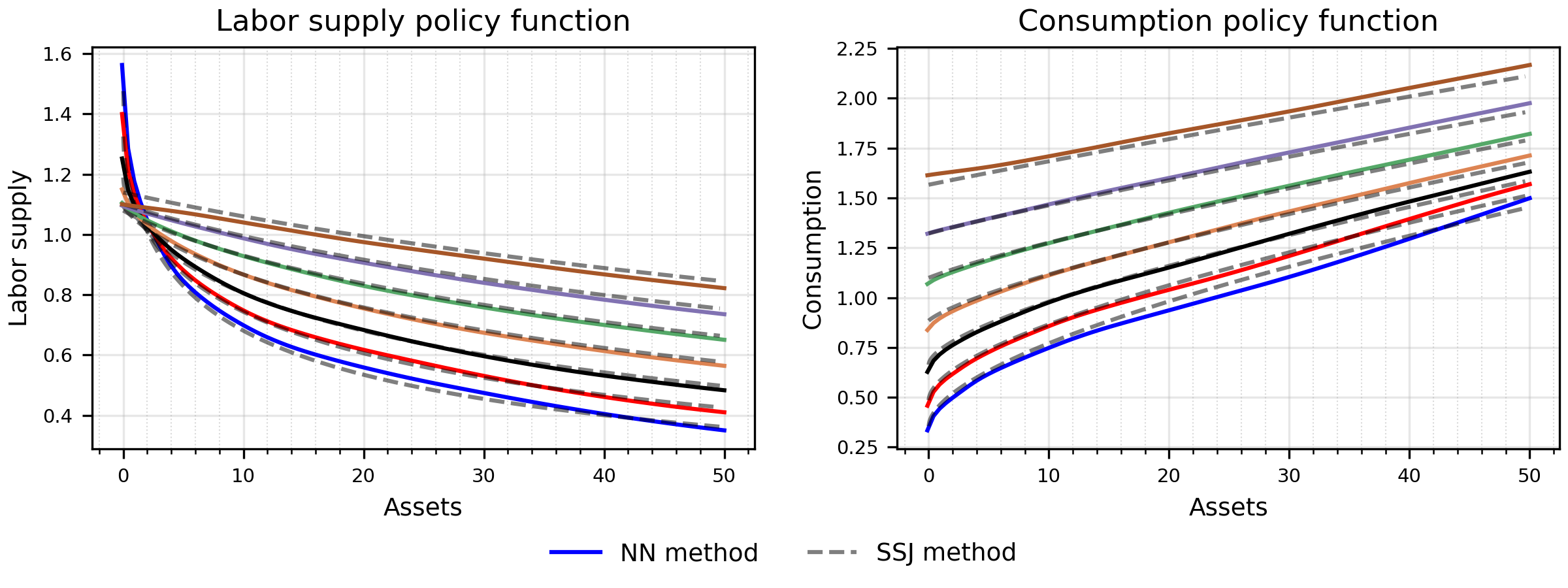
As these households increase savings, the equilibrium interest rate falls. In response, high-productivity households benefit less from working, reduce their labor supply, and increase their consumption. These responses explain why the neural network solution now diverges more substantially from the linearized SSJ solution, which does not account for uncertainty. Part of the gap also comes from the linearization itself, which matters more for larger shocks. In the next figure, the two policy functions of agents now diverge more markedly and for all levels of asset holdings. This is in large part explained by the fact that abstracting from aggregate uncertainty is now consequential.
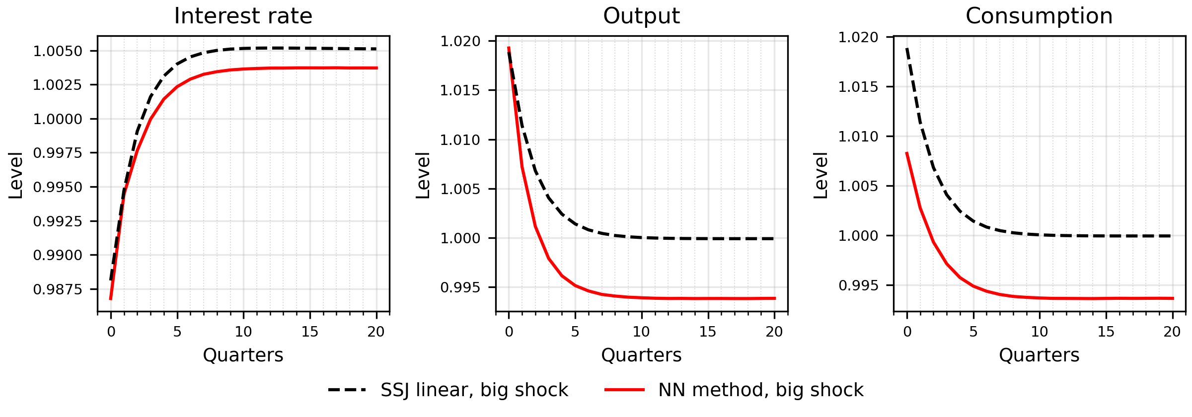
The figure below shows the impulse response functions to a monetary policy shock under high aggregate volatility, approximated using our method (solid red line) and the SSJ method (dashed black line). The responses differ markedly both in the short run and in the long run. The long-run differences can be attributed to the distinct stochastic (risky) steady states, which are captured by our method but not by the SSJ approach.
The differences suggest that when aggregate risk is substantial, as in empirical models, existing methodologies that rely on linearizing aggregate dynamics may fail to accurately capture the impact of uncertainty on the long-run behavior of macro variables and the propagation of shocks. This misrepresentation introduces inaccuracies in the short-run and long-run dynamics of macro observables, which can distort parameter estimates and the model’s predictions.
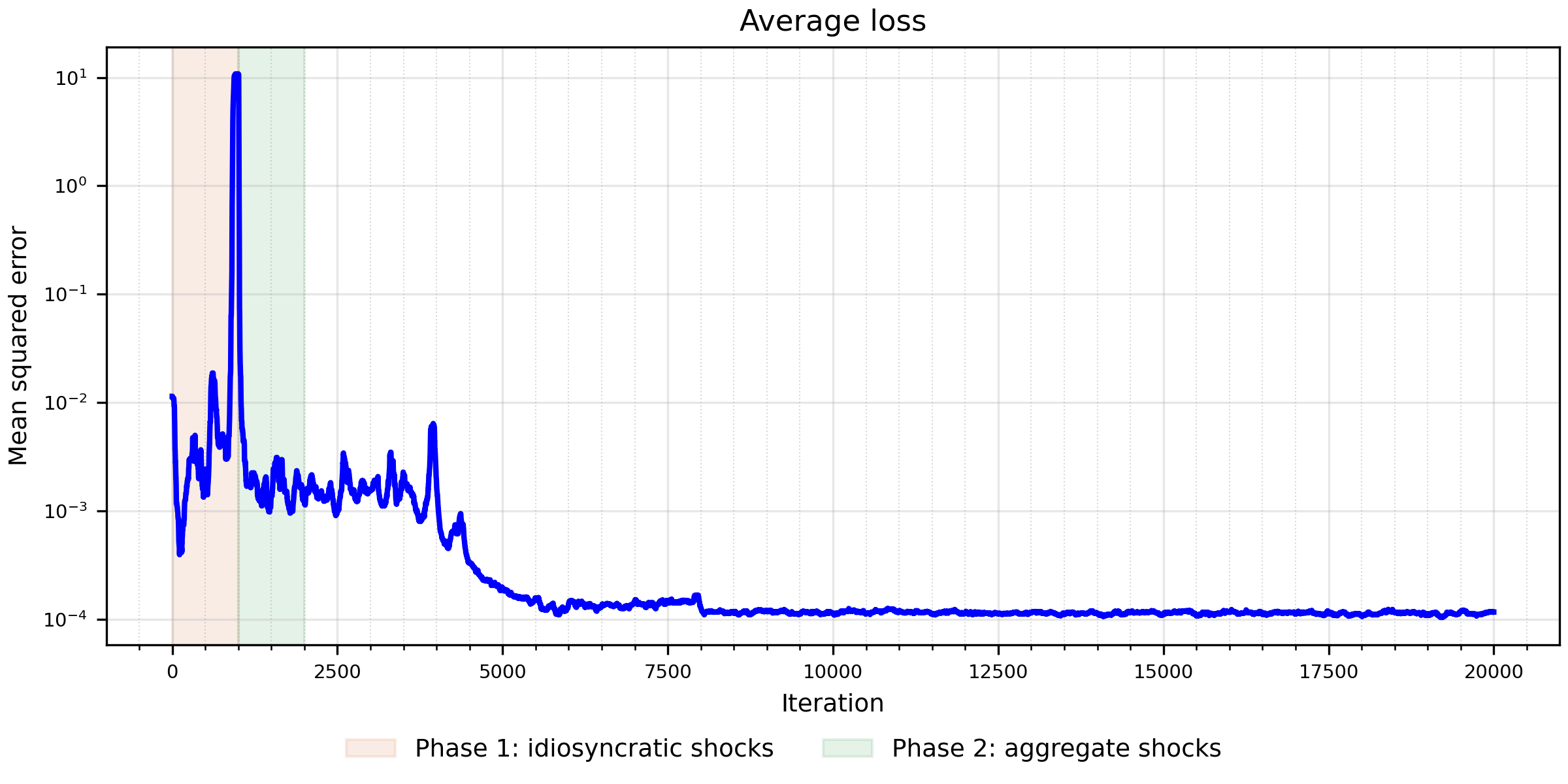
The last figure reports the evolution of the training loss to provide further evidence that the neural-network solution is accurate and reliable. The line reports the loss averaged across the equilibrium conditions that we minimize. The series is calculated as a rolling median over 100 iterations. We facilitate training by initializing the standard deviations of both idiosyncratic and aggregate shocks below their calibrated values and then gradually increasing them to those levels. The shaded areas indicate the phases during which idiosyncratic and aggregate shock volatility, respectively, are gradually scaled up. After the temporary increases associated with these phases, the average loss declines and stabilizes at approximately \(10^{-4}\).
Practical advice in the case of limited access to a GPU
A practical coding strategy leverages the portability of the code architecture through a two-stage approach if there is only limited access to a GPU. During the development stage, the model can be designed and tested on a standard laptop (for example a MacBook, even without using a GPU) using a relatively small number of agents, which enables fast experimentation and debugging. Once the model’s structure and performance are validated, the same code can be executed on a high-performance desktop or server equipped with a GPU. In this implementation stage, the greater computational power allows training neural networks with a much larger number of agents and additional features, thereby improving the precision of the solution and estimation results. This two-stage workflow is particularly useful in practice, as it combines the flexibility and convenience of local model development with the computational efficiency of large-scale implementation, greatly streamlining the research process.